Bottom line: In this Excel formula challenge you will learn how to write a formula to find the first date for each month in a set of data.
Skill level: Intermediate
Video Explanation of the Challenge
Click here to jump down to the Solution Videos
The Competition
Raylene, a member of The Ultimate Lookup Formulas Course (now part of our comprehensive Elevate Excel Training Program), asked a great question about one of the assignments in the course.
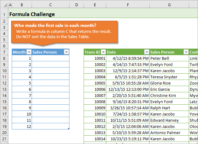
For this challenge, the company's sales team has competition to see who can make the first sale of the month. It's our job to create a report with the list of names for each month's winner.
This task is fairly easy if we can sort the data in the Sales Table. But what if we can't sort it? What would the formula look like then?
Your Challenge
So, my challenge to you is to write a formula in column C to return the name of the sales person that made the first sale in each month.
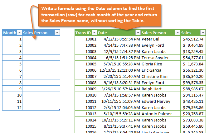
Each row in the Sales Table is a transaction. The Date column (column F) contains the transaction date. Use the Date column to find the first sale for each month of the year, and return the sales person's name from column G.
The only rule is that you cannot sort the Sales Table.
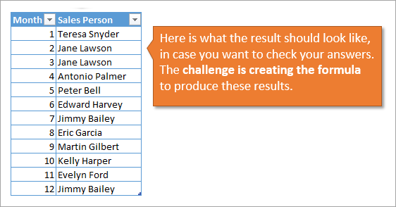
The following image shows the results you are trying to produce. Each name is the first person to make a sale in the month.
Download the Files
Download the Excel file that contains the challenge.
Note about Excel Tables
The file uses Excel Tables. If you're not familiar with Excel Tables yet, you can turn off the structured reference Table formulas, and complete the challenge with regular formula references.
Here is a video on a Beginner's Guide to Excel Tables if you want to learn more about this awesome feature of Excel.
I added a solution file above that uses regular range references ($H$8:$H$1007) instead of structured reference Table formulas (tblSales[Date]). You can use that file if you are not familiar with Table formulas yet.
The Solution Videos
The videos below contain explanations for some of the most popular solutions that were submitted in the comments. The solution file can be downloaded in the section above.
I want to say a big THANK YOU to everyone that participated. We all learned a lot from your solutions.
Here's a link to the playlist of the videos on YouTube if you'd prefer to watch them there.
Video #1: Array Formulas Explained
The most popular solution was using a MIN IF array formula combined with VLOOKUP or INDEX MATCH. In this first video I explain the basics of an array formula. I step through how they calculate on a range of values, and how to use Ctrl+Shift+Enter to enter the formula in Excel.
Video #2: VLOOKUP or INDEX MATCH with MIN IF Array
In this video you will learn how to combine the MIN IF array formula with either VLOOKUP or INDEX MATCH to return the name of the salesperson.
Both techniques return the same result. However, INDEX MATCH is less prone to errors when columns are added/deleted. We can also use INDEX MATCH to return a value to the left of the Date column.
Checkout my free 3-part video series on the lookup formulas to learn more about these awesome functions.
Video #3: The AGGREGATE Function
The AGGREGATE function is a great non-array solution. That means we do NOT have to use Ctrl+Shift+Enter when entering this formula. This is great because most users don't know or understand how to modify array formulas.
For this technique we use the Small function in AGGREGATE to return the smallest value. The Small function has an optional [k] argument that allows us to return the 2nd, 3rd, etc. place value. This makes the formula more versatile if our sales competition gets new rules.
We combine AGGREGATE with VLOOKUP or INDEX MATCH to return the salesperson name.
The AGGREGATE function was introduced in Excel 2010 for Windows, and is available on all Windows and Mac versions after 2010.
Video #4: The New MINIFS Function
The MINIFS function was introduced in Excel 2016 and allows us to calculate a min if based on multiple criteria WITHOUT an array formula. We do NOT have to use Ctrl+Shift+Enter for MINIFS.
It's similar to a SUMIFS or COUNTIFS formula, and is very easy to write. It's probably the easiest solution for this challenge. However, MINIFS is only available on the latest versions of Excel 2016 and you will probably need to be on an Office 365 subscription to get it.
Video #5: Bonus – AGGREGATE with Multiple Criteria
We can also use the same technique with AGGREGATE to calculate a min if based on multiple criteria. This is still a non-array formula, meaning we do NOT have to use Ctrl+Shift+Enter.
And the Winner Is…
Like everything in Excel, there are many ways to solve this problem. This is a great learning experience that should help add a few new techniques to your formula toolbox.
Each solution comes with it's own pros & cons, which I explain in the videos above. I like the AGGREGATE function because of it's availability and versatility.
It's a non-array formula, so we don't have to use Ctrl+Shift+Enter, which is another plus. However, it's still an advanced formula that the average user hasn't seen before. So it will require some explanation if other people are going to be using your file.
MINIFS is the easiest solution, but not widely available if you or your users are on an older version of Excel.
Additional Links Mentioned in the Videos
- How Dates Work in Excel: The Calendar System Explained + Video
- How to Turn OFF Structured References in Excel Table Formulas
- VLOOKUP Example Explained at Starbucks
- VLOOKUP & MATCH: A Dynamic Duo
- The INDEX Function: A Road Map For Your Spreadsheet
- Free 3-part video series on the lookup formulas (VLOOKUP, INDEX, MATCH, & more)
- Free eBook on 10 Excel Formula Pro Tips
Submit Your Answer
Please leave a comment below and paste in your formula solution. There are many ways to go about this, so don't worry if your solution is different from others. This is just a way for everyone to learn from each other.
Also, don't scroll down and look at the other answers until you try it. 😉
Good luck! 🙂


Please leave a comment here and paste in your formula. It will be a great chance to learn from everyone. Thank you! 🙂
Hello Jon, this is my solution:
=INDEX(tblSales[Sales Person],AGGREGATE(15,6,ROW(tblSales[Sales Person])/(tblSales[Date]=AGGREGATE(15,6,tblSales[Date]/(MONTH(tblSales[Date])=[@Month]),1)),1)-ROW(tblSales[[#Headers],[Sales Person]]))
However, if I do it the M-way I discovered a tie in month 4: Samuel Vasquez and Antonio Palmer.
actually this is the best i used it many times in reports
Ciao Jon!
I came up a slightly shorter solution which got to be entered as an array formula with CTRL+SHIFT+ENTER. Namely:
=INDEX(tblSales[Sales Person],MATCH(MIN(IF(MONTH(tblSales[Date])=B8,tblSales[Date],””)),tblSales[Date],0))
How does the formula work?
==========================
I found the earliest date entry in the “Date” column of the sales table “tblSales” of which MONTH value is equal to the current month in cell B8.
Then I retrieve the position number of this date entry in the tblSales[Date] column using EXACT MATCH.
Using this position number, I retrieve the salesperson’s name with the INDEX() function. In other words, I search for the name of that particular salesperson in the tblSales[Sales Person] column who is listed in the same position as the one retrieved earlier using EXACT MATCH.
I have four embedded functions in my formula:
=INDEX(Sales Person Column, MATCH( MIN( IF(…) ),Date Column,ExactMatch) ))
Ciao & cheers!- D/A
How come it does not work for me? I get “NAME?” error when using your formula.
Since the only rule is that the data cannot be sorted, I would add a column to the sales table to extract the month. The formula to return the Sales Person would then be:
=VLOOKUP(MINIFS(tblSales[Date],tblSales[Month],[@Month]),tblSales[[Date]:[Sales Person]],2,FALSE)
That is the exact sale solution I came up with Gwebbo.
Since we know the result set is for a specific year (2015, in this case) we can use a pretty simple formula (as long as you have Excel 2016, which introduced the MINIFS formula).
=INDEX(tblSales[Sales Person], MATCH(MINIFS(tblSales[Date], tblSales[Date], "="&DATE(2015, [@Month], 1)), tblSales[Date], 0))
So, we index the ‘Sales Person’ field in the tblSales table and match it to the relative row of the minimum date that is less than the “first of next month”, but greater than or equal to the “first of this month”.
The largest flaw in this solution is that if there were any ties, they would be solved by simply returning the first name that equals the minimum timestamp (so, sort order would matter), but I’m not aware of any way for Excel to return a tie outside of using VBA (which defeats the purpose of this exercise).
Hey Jon,
Here is what I came up with:
=INDEX(tblSales,MATCH(MIN(IF(MONTH(tblSales[Date])=[@Month],tblSales[Date],FALSE)),tblSales[Date],0),3)
Thanks
My solution is pretty simple, but does rely on having Excel 2016, which introduced the “MINIFS” formula:
=INDEX(tblSales[Sales Person], MATCH(MINIFS(tblSales[Date], tblSales[Date], “=”&DATE(2015, [@Month], 1)), tblSales[Date], 0))
So, I’m indexing the tblSales ‘Sales Person’ field and returning the relative row of the minimum date which is greater than or equal to the “first day of THIS month” and less than the “first day of NEXT month”. Of course, this formula also assumes that this data would be kept for “each year”. The easy solution to a situation where you would want multiple years would be to store the Month in tblFirstSale as 1-1-YYYY and format the display to show the “m” only and reference [@Month] in the formula above.
The only flaw is that this does not break any ties – it would depending on the sorting logic of the tblSales table and would simply return the first match. Outside of using VBA (which is outside the scope of the challenge), I am not aware of any way to return both rows.
Does this actually work, it returns #N/A to me. Also, June does not have data for the 1st, wouldn’t the above return blank?
He just left out the “greater than” sign. The formula should have “>=” instead of “=”.
The quickest in my opinion is a pivot table, with a formula to check for change in the months. (but not sure if that is allowed)
Years Months Days Hours Date Sales Person
2015 Jan 01-Jan 15 :27 Teresa Snyder 1
2015 Feb 01-Feb 00 :22 Jane Lawson 1
2015 Mar 01-Mar 15 :49 Jane Lawson 1
2015 Apr 01-Apr 17 :38 Antonio Palmer 1
2015 May 01-May 01 :02 Peter Bell 1
2015 Jun 02-Jun 03 :39 Edward Harvey 1
2015 Jul 01-Jul 01 :12 Jimmy Bailey 1
2015 Aug 01-Aug 06 :55 Eric Garcia 1
2015 Sep 01-Sep 02 :14 Martin Gilbert 1
2015 Oct 01-Oct 08 :48 Kelly Harper 1
2015 Nov 01-Nov 03 :13 Evelyn Ford 1
2015 Dec 01-Dec 02 :12 Jimmy Bailey 1
Grand Total
In C8 -> =VLOOKUP(MIN(IF(MONTH(tblSales[Date])=[@Month],tblSales[Date])),tblSales[[#All],[Date]:[Sales Person]],2,0)
Ctrl-Shift-Enter
Hello Jon, this is my solution:
=VLOOKUP([@Month],G:H,2,FALSE)
Then i check my answer for first sales person every month is exactly the same after i filtering to double check the answer.
Thanks.
Hi Jon,
Love the site, keep up the great work! My solution involved using an array formula (and a fairly safe assumption that all dates run prior to Nov. 26, 4637):
{=VLOOKUP(MIN(IF([@Month]=MONTH(tblSales[Date]),tblSales[Date],1000000)),tblSales[[Date]:[Sales Person]],2,0)}
The 1,000,000 qualifier is arbitrary, just used to ensure MIN() will only consider the minimum date/time for the desired month.
Mine is an array formula:
{=VLOOKUP(MIN(IF(MONTH(tblSales[Date])=[@Month],tblSales[Date])),tblSales[[Date]:[Sales Person]],2,0)}
Pls hit CTRL + SHIFT + ENTER
There is tie between Antonio Palmer & Samuel Vasquez for the month of April.
=INDEX(G8:G1007,MATCH(MIN(IF(MONTH(F8:F1007)=B8,F8:F1007)),F8:F1007,0))
array-entered in C8
Why is my comment not shown?
Hi Rudra,
The comments must be approved and then take a little time to show due to the site caching. So don’t worry if you don’t see your comment yet, we received and it will appear soon. Thanks for participating! 🙂
Hi Jon,
Here is my solution:
={VLOOKUP(MIN(IF(MONTH(tblSales[Date])=[@Month],tblSales[Date])),tblSales[[#All],[Date]:[Sales Person]],2,0)}
Array formula was used.
Hi
I tried using Hepler Column:
=INDEX(tblSales2[[#All],[Sales Person]],MATCH(CONCATENATE(CHOOSE(B8,”Jan”,”Feb”,”Mar”,”Apr”,”May”,”Jun”,”Jul”,”Aug”,”Sep”,”Oct”,”Nov”,”Dec”),”|”,1),tblSales2[[#All],[Unique Key]],0))
Hi Jon,
Used this two formulas:
=INDEX(tblSales[Sales Person],MATCH(MIN(IF(MONTH(tblSales[Date])=tblFirstSale[@Month],tblSales[Date])),tblSales[Date],0))
=VLOOKUP(MIN(IF(MONTH(tblSales[Date])=[@Month],tblSales[Date])),tblSales[[#All],[Date]:[Sales Person]],2,0)
And applied the array formula method (Ctrl+Shift+Enter)
This seems to do the trick (as an array formula):
{=INDEX(tblSales[Sales Person],
MATCH(MIN(IF((MONTH(tblSales[Date])=tblFirstSale[@Month])*(tblSales[Date])
0,tblSales[Date])
),
tblSales[Date],
0)
)}
{=VLOOKUP(MIN(IF(MONTH(tblSales[Date])=[@Month],tblSales[Date])),tblSales[[Date]:[Sales Person]],2,FALSE)}
A short array formula:
{=VLOOKUP(MIN(IF(MONTH(tblSales[Date])=[@Month],tblSales[Date])),tblSales[[Date]:[Sales Person]],2,FALSE)}
Probably not as elegant as some others, but it works when entered as an array (CTRL-SHFT-ENTER)
=VLOOKUP(MIN(IF(MONTH(tblSales[Date])=$B8,tblSales[Date])),tblSales[[Date]:[Sales Person]],2,0)
{=INDEX(tblSales,MATCH(MIN(IF(MONTH(tblSales[Date])=INDEX(B:B,ROW()),tblSales[Date])),tblSales[Date],0),3)}
Must be entered as an array formula!
Hi Jon
Here is our formula, but it must be activated with Ctrl+Shift+Enter to work with arrays:
=VLOOKUP(MIN(IF([@Month]=MONTH(tblSales[Date]),tblSales[Date])),tblSales[[Date]:[Sales Person]],2,FALSE)
This is my second submission since I did not see my earlier one posted. This works when entered as and array (CTRL-SHIFT-ENTER)
=VLOOKUP(MIN(IF(MONTH(tblSales[Date])=$B8,tblSales[Date])),tblSales[[Date]:[Sales Person]],2,0)
Hi Jon,
I think this is the best solution.. 🙂
=VLOOKUP(SMALL(tblSales[Date];[@Month]);tblSales[[Date]:[Sales Person]];2;FALSE)
Hi,
Here’s my solution an array formula:
=INDEX(tblSales[Sales Person],MATCH(MIN(IF(MONTH(tblSales[Date])=[@Month],tblSales[Date])),tblSales[Date],FALSE))
I did it with a Power Query query and I had a tie also in April
Hello,
it might be very wrong, but here is my solution to this:
{=INDEX(tblSales[Sales Person],MATCH(MIN(IF(MONTH(tblSales[Date])=[@Month],tblSales[Date])),tblSales[Date],0))}
And i will have to agree with XLarium for April sorting the data we have a tie between:
10018 4/1/15 5:38:53 PM Antonio Palmer
10023 4/1/15 5:38:53 PM Samuel Vasquez
Will gladly look at the solutions others may have, and of course yours Jon!
Best regards
{=VLOOKUP(MIN(IF(MONTH(tblSales[Date])=[@Month],tblSales[Date])),tblSales[[Date]:[Sales Person]],2,0)}
Hi Jon, here’s my solution:
=INDEX(tblSales[Sales Person],MATCH(SMALL(tblSales[Date],COUNTIF(tblSales[Date],”<"&DATE(2015,[@Month],1))+1),tblSales[Date],0))
Have never used the SMALL function before this but it proved very useful here.
=INDEX(tblSales[Sales Person],MATCH(SMALL(tblSales[Date],COUNTIF(tblSales[Date],”<"&DATE(2015,[@Month],1))+1),tblSales[Date],0))
This is how I solved it, have never used the SMALL function before but it was useful here.
Hi Jon,
I used an array formula:
{=INDEX(tblSales[Sales Person],MATCH(SMALL(IF(MONTH(tblSales[Date])=[@Month],(tblSales[Date])),1),tblSales[Date],0))}
Hi Jon,
My formula would be an array formula:
{=INDEX(tblSales[Sales Person],MATCH(SMALL(IF(MONTH(tblSales[Date])=[@Month],tblSales[Date],””),1),tblSales[Date],0))}
I have added the {} to the above to clarify that it is an array.
I added a couple of columns with the following formulas: –
Column J (titled Month) =MONTH([@Date])
Column K (Titled DateNumber, formatted as number) =VALUE([@Date])
Column L (titled Check) = {=IF(MIN(IF(Months=J8,Dates))=K8,J8,0)}
and in the table required formula :
=INDEX(tblSales[[#All],[Sales Person]],MATCH([@Month],tblSales[[#All],[Check]],0))
Here we go, that was fun!
=INDEX(tblSales[Sales Person],MATCH(MIN(IF(MONTH(tblSales[Date])=[@Month],tblSales[Date],FALSE)),tblSales[Date],0),1)
This is what I came up with.
{=VLOOKUP(MIN(IF(MONTH($F$8:$F$1007)=B8,$F$8:$F$1007)),$F$8:$G$1007,2,FALSE)}
Hi Jon & XLarium & Everyone,
Here is my array:
=INDEX(tblSales3[Sales Person],MATCH(MIN(IF(MONTH(tblSales3[Date])=[@Month],tblSales3[Date],””)),IF(MONTH(tblSales3[Date])=[@Month],tblSales3[Date],””),0))
Thanks for the Excel puzzle Jon!
Cheers,
Kevin
It’s ugly but works. Picks the first person in the list in case of tie. I’ll need to add a tie breaker based on the highest sales.
{=INDEX(tblSales[Sales Person],MATCH(SMALL(IFERROR(tblSales[Date]*(1/(MONTH(tblSales[Date])=[@Month])),””),1),tblSales[Date],0))}
Here you go:
=INDEX(tblSales[Sales Person],MATCH(MIN(IF(MONTH(tblSales[Date])=[@Month],tblSales[Date],””)),tblSales[Date],0))
Used as an Array of course.
Cheers,
Adrian
Got it!:)
=VLOOKUP(MIN(IF(MONTH(tblSales[Date])=[@Month],tblSales[Date],””)),tblSales[[Date]:[Sales Person]],2,FALSE)
=VLOOKUP(MINIFS($F$8:$F$1007,$F$8:$F$1007,”=”&DATE(YEAR($F$8),B8,1)),$F$8:$G$1007,2,FALSE)
Relies on year in the first row of data as well as MINIFS function from Office 2016/365.
Very good way for users to learn formula. This is great initiative.
@XLarium
I checked your formula does not produce correct result. for Feb it returns Jane Lawson while the the correct value to return is Evelyn Washington
Thanks for the feedback, Jamil M.
According to Jon it should be Jane Lawson for Feb (see in article above). So the formula returns the correct value.
Maybe Jon did some changes to the file in the meantime that would present Evelyn Washington as a correct solution for Feb.
Yes, in that case it is correct.
It is a good one as it doesn’t require CSE
I’ve got this – array formula (CSE entered):
=INDEX(tblSales[Sales Person],MATCH(MIN(IF(MONTH(tblSales[Date])=[@Month],tblSales[Date],”A”)),tblSales[Date],0))
Then realised it was basically the same as Deniz Aksen’s. Hey ho!
=INDEX(tblSales[Sales Person],MATCH(MIN(IF(MONTH(tblSales[Date])=[@Month],tblSales[Date])),tblSales[Date],0))
Another way you can get the result by using LOOKUP function.
with CSE
=LOOKUP(2,1/(MIN(IF((MONTH(tblSales[Date])=[@Month])*tblSales[Date]>0,(MONTH(tblSales[Date])=[@Month])*tblSales[Date]))=tblSales[Date]),tblSales[Sales Person])
Hi Jon,
This is my solution with an array formula:
{=INDEX(tblSales;MATCH(MIN(IF(MONTH(tblSales[Date])=[@Month];tblSales[Date];MAX(tblSales[Date])));tblSales[Date];0);3)}
Is close to the one of Deniz.
BTW – Working with Excel 2016 which has no clue about MINIFS… 🙂
Jon,
My solution:
=ÍNDEX(tblSales[Sales Person];CORRESP(MIN(IF(MONTH(tblSales[Date])=B8;tblSales[Date]);1);tblSales[Date];0))
this is a matrix formula, i.e. to be confirmed with Ctrl + Shift + Enter:
{=INDEX(tblSales[Sales Person],MATCH(MIN(IF(MONTH(tblSales[Date])=[@Month],tblSales[Date],””)),tblSales[Date],))}
Hi Jon,
I’m in the habit of trying to avoid array formulas because no one else in my office knows what they are or how they work. That added another level of challenge. I also noticed that there was a TIE for the first sale in April, and it wasn’t specified if the first transaction ID was actually first, so I built in a contingency for a tie, to return the two people who technically could have had the first sale based on the date/time stamp.
Here is the formula for C8:
=IF(COUNTIF(tblSales[Date],MINIFS(tblSales[Date],tblSales[Date],”>=”&DATE(2015,B8,1)))>1,CONCATENATE(COUNTIF(tblSales[Date],MINIFS(tblSales[Date],tblSales[Date],”>=”&DATE(2015,B8,1))),”-Way Tie Between “,INDEX(tblSales[#All],MATCH(MINIFS(tblSales[Date],tblSales[Date],”>=”&DATE(2015,B8,1)),tblSales[[#All],[Date]],0),MATCH(tblFirstSale[[#Headers],[Sales Person]],tblSales[#Headers],0)),” & “,INDEX(tblSales[#All],MATCH(MINIFS(tblSales[Date],tblSales[Date],”>=”&DATE(2015,B8,1)),tblSales[[#All],[Date]],0)+MATCH(MINIFS(OFFSET(tblSales[Date],MATCH(MINIFS(tblSales[Date],tblSales[Date],”>=”&DATE(2015,B8,1)),tblSales[[#All],[Date]],0),0),OFFSET(tblSales[Date],MATCH(MINIFS(tblSales[Date],tblSales[Date],”>=”&DATE(2015,B8,1)),tblSales[[#All],[Date]],0),0),”>=”&DATE(2015,B8,1)),OFFSET(tblSales[[#All],[Date]],MATCH(MINIFS(tblSales[Date],tblSales[Date],”>=”&DATE(2015,B8,1)),tblSales[[#All],[Date]],0),0),0),MATCH(tblFirstSale[[#Headers],[Sales Person]],tblSales[#Headers],0))),INDEX(tblSales[#All],MATCH(MINIFS(tblSales[Date],tblSales[Date],”>=”&DATE(2015,B8,1)),tblSales[[#All],[Date]],0),MATCH(tblFirstSale[[#Headers],[Sales Person]],tblSales[#Headers],0)))
Breaking it down –
The first step was to identify the date of the first sale in the given month. I used the minifs function to identify the smallest date which was greater than or equal to the date with 2015 as the year, the variable in column B as month, and the 1st as the day.
The second step was to use an index match to find that date and return the Sales Person.
The third step (which if I was Samuel Vasquez I would protest heavily was missing!!!) was to check to see if there were any repeating dates/times that would indicate a tie. I used the count function to test if the smallest date I found was unique. If it WASN’T unique, a x-way tie was identified, and I used concatenate to return a count of duplicate values (x), the name of the first salesperson I had already found, and the name of the second with the repeated date. Since I decided not to use an array formula, I used “offset” to set the index range just below the first match value for the second match. Technically this formula could be expanded to accommodate a 3-way, 4-way, ect tie, but I figured since a 2 way tie was rare enough, it would be enough for the formula to identify any “x-Way Tie Between”s and for someone to manually enter any additional names beyond the first two (rather than further over complicate the formula).
Thanks for the challenge 🙂 Love this stuff!!
{=INDEX($G$8:$G$1007,MATCH(SMALL(IF(MONTH($F$8:$F$1007)=B8,$F$8:$F$1007),1),$F$8:$F$1007,0))}
Since XLarium and Mara noted that there was a tie in April, I thought I would use the largest sales amount to break the tie. It is just a coincidence that most of these formulas choose Palmer as the winner in April. They are just taking the first row that has the date of the tie, and Palmer whose sale was $72k, WAS the larger sale for that date/time.
Unfortunately, if you exchange the Trans ID on these two rows; 10018 and 10023, and resort so that Vasquez with $42k in sales is first, he shows up as the winner.
My solution uses Kent’s formula to find the twelve minimum dates, but then goes on to find all the rows with those sales dates and times and chooses the row with the highest sales each month. Using this additional rule, Palmer IS the legitimate winner in April.
Although Kent’s formula is not an array formula, this one only works if you use ++ since it does a secondary search to find all records with the winning date and time each month.
I used R1C1 style of reference for the INDIRECT function since the Sales table might not always be in the same location. E.g., I had inserted some columns to the left of it so that I could insert some of the best answers from other people on this challenge.
Here is the formula:
{=INDIRECT(“R”&MATCH(INDEX(tblSales[Date], MATCH(MINIFS(tblSales[Date], tblSales[Date],”>=”&DATE(2015, [@Month], 1)), tblSales[Date], 0))&MAX(IF(INDEX(tblSales[Date], MATCH(MINIFS(tblSales[Date], tblSales[Date],”>=”&DATE(2015, [@Month], 1)), tblSales[Date], 0))=tblSales[Date],tblSales[Sales],””)),tblSales[Date]&tblSales[Sales],0)+7&”C”&COLUMN(tblSales[[#Headers],[Sales Person]]),0)}
Please replace + + in the fourth paragraph. It should say this is an array formula and needs to be entered with Ctrl + Shift + Enter to work.
I should probably make the MAX sales search dynamic for row placement, too. We can make this happen if we replace the +7 near the end of the formula. That constant accounts for the blank rows above the Sales table. Replace +7 with: +ROW(tblSales[[#Headers],[Trans ID]]) to allow placement of the table at any spot on the sheet.
Here is another formula that breaks ties by choosing the highest sales amount on the winning date:
{=INDEX(tblSales[Sales Person], MATCH(MINIFS(tblSales[Date], tblSales[Date],”>=”&DATE(2015, [@Month], 1))&MAX(IF(INDEX(tblSales[Date], MATCH(MINIFS(tblSales[Date], tblSales[Date],”>=”&DATE(2015, [@Month], 1)), tblSales[Date], 0))=tblSales[Date],tblSales[Sales],””)), tblSales[Date]&tblSales[Sales], 0))}
Remember to enter Ctrl + Shift + Enter since this is a MATCH array formula – it matches both the earliest sale date in the month and the highest sales amount on that date.