The INDEX function is commonly used in combination with the MATCH function to provide powerful and dynamic lookup formulas.
This post will just focus on explaining the how the INDEX function works. It is best to understand the basics of INDEX before creating more advanced formulas using INDEX & MATCH.
Series: The Lookup Functions Explained
This is the third post in a series about the most commonly used lookup functions in Excel.
- In the first post I explained the VLOOKUP function at Starbucks.
- The second post explained how to make lookup formulas more dynamic with the VLOOKUP & MATCH functions.
- In this third post I will explain the INDEX function.
The INDEX Function is a Road Map
The INDEX function always reminds me of reading a road map.
As a kid, I had a fascination with maps. My parents always let me be the “navigator” on long road trips, and my job was to figure out where we were going and follow our course on the map.
The old road maps were laid out in a grid with columns and rows, just like an Excel spreadsheet.
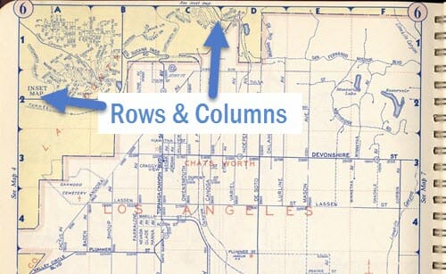
You would first have to find the coordinates of your destination in the index of the map book, then locate the page and grid square (cell) that your destination was in.
The INDEX function in Excel is very similar to this. Its job is to return a cell value based on the grid coordinates that you feed it.
It is a very simple function.
I believe it has a reputation for being difficult and confusing because you have to combine it with a MATCH function to use it as a lookup formula.
So we are just going to start with the basics of how the INDEX function works.
Download the Example File
Please fill out the form below to download the example files immediately.
The INDEX Function Explained
The INDEX function returns the value of a cell based on the grid coordinates you provide it.
There are three arguments to the INDEX function.
=INDEX(array, row_num, [column_num])
Let’s look back at our Starbucks menu example to learn about the arguments in the INDEX function. This time we will use the INDEX function to answer the same question from the VLOOKUP example.
“What is the price of the Caffe Mocha, size Grande?”
1. array – This is the where argument.
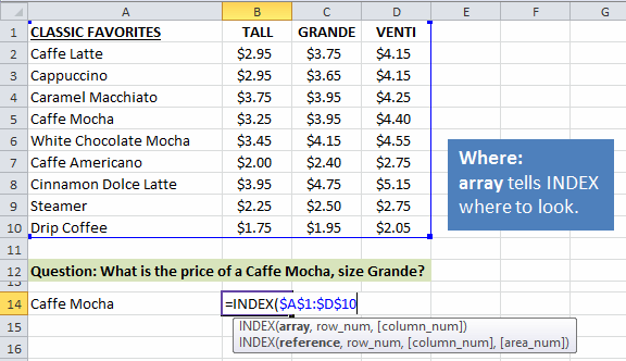
This argument tells the INDEX where we want to look in the spreadsheet. You specify a range like A1:D10.
To me this is very similar to the page in the map book. We first need to tell INDEX where we are going to look, then zoom in on the exact coordinates.
The next two arguments are the coordinates.
2. row_num – This is the row number of the array that we want to return the result from.
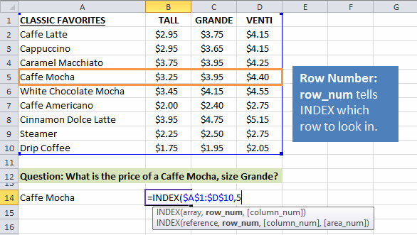
In our example, we want to return a result from row 5. Since Caffe Mocha is in row 5 of the array, we simply put a 5 in the second argument of the formula.
3. column_num – This is the column number of the array that we want to return the result from.
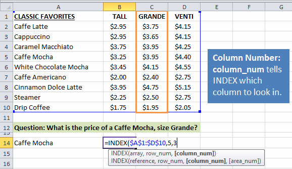
We know that we want to return a price from the size Grande column, which is in column 3 of the array. So we can put a 3 in the third argument of the function.
The Result
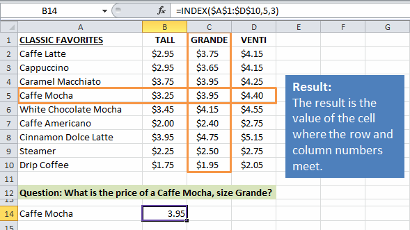
The INDEX formula returns the result: $3.95. This is the value of cell C5 in the worksheet.
I hope this helps explain how simple the INDEX function is. You just tell it where you want to look (the array), and then give it the coordinates (the row & col numbers) of the cell value you want to return.
Row and Column Numbers are Relative to the Array Range
One important thing to note is that the row and column numbers we used in the INDEX function are relative to the array range ($A$1:$D$10).
In the example above we used row 5 and column 3 in the INDEX function. This is NOT necessarily the row and column number of the worksheet. The array range in our formula starts in cell A1, so the column and row number of the array will be the same as the column and row number of the worksheet.
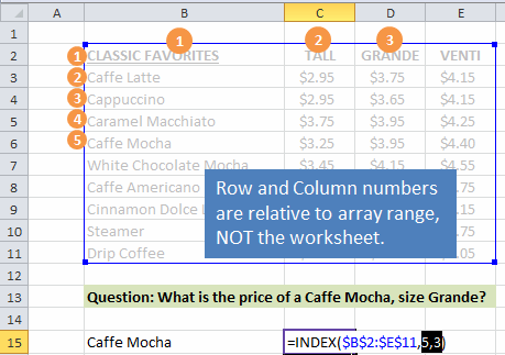
If however, the array range started in cell B2, then the array range would be $B$2:$E$11. The price for the Caffe Mocha size Grande would still be in the 5th row and 3rd column of the array range. Therefore, the row and column arguments in the formula would remain 5 and 3.
You can see that the column and row numbers are specific to the array range, NOT the worksheet.
Conclusion
This should give you a basic understanding of how the INDEX function works.
It also explains that 20 years later, my fascination for maps and grids has not changed. 🙂
In the next post in this series I will discuss how the INDEX and MATCH functions can be combined to create powerful lookup formulas that can have advantages over the traditional VLOOKUP.
Additional Resources
Here are links to the other two posts in this series about LOOKUP functions.
Please leave a comment below with any questions.
Take the VLOOKUP Challenge
I've put together 5-part video training series that will help you learn more about lookup formulas and test your skills.


thank you for the post, i had trouble understanding how the index function works, until now. you have a great way of translating formula terms into terms i can understand.
Thank you for the nice comment Angela! I’m so glad you found it useful. Let me know if you have any other questions about INDEX, or anything else.
Did you end up posting the tutorial on index + match?
Hi Brian,
I don’t have a tutorial on Index & Match yet. I do have an article on Vlookup & Match. This explains how the Match function works to return a row or column number. It’s best to learn how the Match function works before combining it with Index. With that said, I definitely need to write an article on Index & Match. I will notify everyone on my free email newsletter when it is available. Thanks!
Hello Jon, I find your instruction style very effective. I too am looking for the INDEX/MATCH tutorial. Thanks Roland
Dear Jon,
I can,t wait to read the next post. Please do it sonnest.
Hi, Jon:
This is Mary from Epicor APAC. I wish I had known your excellent blog earlier!
Questions as following:
1. I cannot find your next post below.
In the next post in this series I will discuss how the INDEX and MATCH functions can be combined to create powerful lookup formulas that can have advantages over the traditional VLOOKUP.
2. I had difficulty to download your free book.
Thanks, Jon !
Mary
Hi Mary! Great to see you here! To answer your questions:
1. I have not written that post yet, but I will definitely let you know when it is available.
2. I’m sorry you had difficulty downloading the book. I’m looking into changing that process to make the whole thing easier.
Thanks for letting me know Mary!
Happy New Year!
It’s informative, useful… thanks for posting.
Waiting for your post on INDEX MATCH. It is informative and captivating too please.
I used to use VLOOKUP all of the time until I discovered how INDEX MATCH easily overcomes all of the drawbacks of VLOOKUP when you are adding or removing columns to the worksheets from which you are looking up your desired results.
One of the key differences with INDEX MATCH is that, rather than selecting an entire array table, you are only selecting the lookup column and the return column of what would be a VLOOKUP array. While not a big deal when it comes to simple lookups, this can definitely become a factor if you are dealing with large files that have thousands of lookups. By limiting your arrays to only the lookup and return columns, you reduce the processing load on Excel.
The other key difference is that INDEX MATCH formulas work as a right to left lookup, whereas VLOOKUP only works left to right. As you can see in the example below, I can use INDEX MATCH to lookup a value that is to the right of my return value using INDEX MATCH. This is not possible with the VLOOKUP formula, as you would have to rearrange your data set, or copy your lookup column so that it is always to the left of your return value.
Here’s how I think about the INDEX MATCH formula as I’m typing it in:
=INDEX(Column containing the results I want to appear in this cell,MATCH(Cell in this row containing the value to lookup,Column containing the matching value being looked up,FALSE),1)
So this VLOOKUP formula:
=VLOOKUP(A5,’Max $ Limitation Lookup’!A:AZ,48,FALSE)
Would become this INDEX MATCH formula:
=INDEX(‘Max $ Limitation Lookup’!AV:AV,MATCH(A5,’Max $ Limitation Lookup’!A:A,FALSE),1)
Initially the INDEX MATCH formula looks more complicated, but the advantage is that the INDEX MATCH formula has no problem with me deleting or adding any number of columns on the ‘Max $ Limitation Lookup’ worksheet as long as I don’t delete the columns containing my results or my lookup values.
I even proceeded to create a spreadsheet named “Convert VLOOKUP To INDEX MATCH.xlsx” and used it to convert all of the VLOOKUP formulas in all of my spreadsheets to INDEX MATCH formulas. It automatically converts a pasted VLOOKUP formula to an INDEX MATCH formula that can be copied and pasted back to the source spreadsheet.
I would love to share my “Convert VLOOKUP To INDEX MATCH.xlsx” spreadsheet with you if you would like to have it and/or share it.
Hi Bill,
Thanks for taking the time to write and share your experience. I just published a free video series on the lookup formulas including VLOOKUP and INDEX/MATCH, and I discuss a lot of these points as well. INDEX/MATCH has a few advantages over VLOOKUP that make it more flexible and less prone to errors.
I would be happy to checkout your file and post it here. You can send it to me at [email protected]. Thanks again!
Hi Jon,
Great website with cool tutorials.
While Reading this Index funtion example a question popped into my mind considering the arguments shown.
In the example “=INDEX(array, row_num, [column_num])” if the row_num and [column_num] were 5 and 3 respectively, why aren’t those arguments written as 5 and [3] if the column_num is within []?
Thanks,
Rui
Hi Rui,
Great question! The square brackets [] indicate that the argument is optional. This means it is NOT required. If there was only one column in the array then we could use the following formula.
=INDEX(A1:A10,5)
The column_num argument does not need to be specified and can just be left blank.
This rule applies to all functions in Excel. When you see the argument name in square brackets that means it is optional. Some optional arguments default to a certain value. For example, the last argument in vlookup defaults to TRUE if you don’t specify it.
I hope that helps. Thanks!
Well done, and very clearly explained. Thanks, Jon.
Thanks Jon,
Just thinking if the INDEX function is the best for large data sets with 1,000s of rows and numerous columns. Is there a way combining the capabilities of VLOOKUP and INDEX? This way Excel will help search a certain value down numerous rows and match it with another in a specified column.
Best,
Munya.
Hi Jon,
Create job at explaining these functions very simply and giving the understanding behind it all.
I love your analogies also.
Excellent!!
Susanne
Hey Jon
Loved your explanation!
Any chance you will upload your article on INDEX and MATCH functions combined?
Jose
Thanks Jose! Yes, we are working on a new video and article for INDEX and MATCH right now. Should be out in the next few weeks. Stay tuned. 🙂
I have gotten important things thank you.
Thanks a tonne for your help! Can’t even tell you beneficial these were 🙂
This was great, thank you so much! Common errors helped me troubleshoot my first mistake very quickly so thank you for that detail!
Love your work sir. Straight to the point.
Hello Brain,
Superb explanation on index I would like to know if in the cell if there are blanks i want to know only data present in the cell example :
User ID jan Feb Mar Apr May Jun Jul
0001 23 56 70 81 89 45
0002 31
0003 123 131 12 312 313 13
in the above table, I just want to know in which month the user has logged in the month name should be shown like 0001 user has logged in month Feb kindly help me providing solution on it.
Thank you for the explanation. This is so helpful