VLOOKUP & MATCH – A Dynamic Duo

This post provides an explanation of how to use the VLOOKUP and MATCH functions to give you better control over how the column index number changes.  This is often referred to as a dynamic formula.  You will learn how this dynamic duo can help prevent errors and improve your VLOOKUP formulas.

The Dynamic Duo

We are going to learn how the MATCH function can be used inside the VLOOKUP function.  This helps protect the VLOOKUP from returning errors when changes are made to the workbook.

Problems with VLOOKUPs

The VLOOKUP is a very useful function, but it doesn't respond to change very well.  Have you ever noticed that if you add or delete columns in an area that the VLOOKUP refers to, the result can return an error or incorrect result?

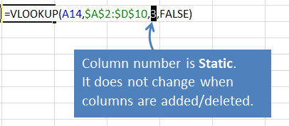
This is usually due to the fact that we have specified the column number as a static number in the 3rd argument of the VLOOKUP argument.

The Starbucks Menu Example

We can use the Starbucks menu VLOOKUP example to help explain this issue.

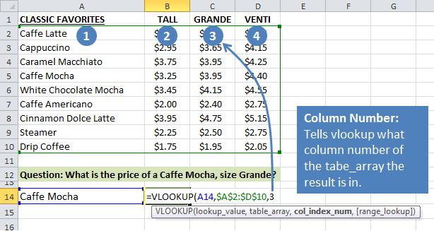
In that example we wanted to return the price for the size Grande, which was in column 3 of the menu.  We put a “3” in the column index argument in the VLOOKUP formula to reference the Grande column (col C).

But what if Starbucks decided to add a new size to the menu?

Let's say they decide to add a size “Short” to the menu, and put it to the left of the size Tall.

In our spreadsheet example, we would need to insert a column after column A for the new size.  This change means that the size Grande is now in column 4 (col D).

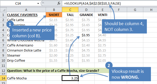
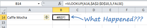
However, our VLOOKUP still references column 3.  Excel does NOT update the formula when a column is inserted or deleted.

Therefore, the formula is now returning the wrong result.

This is a problem!  But fortunately for us, VLOOKUP has a side-kick named MATCH that will save the day.

MATCH to the Rescue

We first need to learn how the MATCH function works.

The MATCH function is very similar to the VLOOKUP.  It's job is to look through a range of cells and find a match.

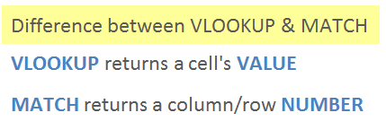
The difference is that it returns a row or column number.

So why the Batman and Robin reference?

I like to think of MATCH as VLOOKUP's little brother, or side-kick.  They do very similar jobs, but MATCH packs a smaller punch.

Batman is the VLOOKUP and returns a big value in the form of a cell's value.  This can be text or a number.

Robin is the MATCH and returns a smaller value in the form of a number.

Hopefully this will help you remember and distinguish the difference between the two.

The Match Function Components

The MATCH function's arguments are similar to the VLOOKUP's.  The following image shows the Excel definition of the VLOOKUP function, and then my simple definition.  This simple definition just makes it easier for me to remember the three arguments.

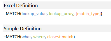
I explain this simple definition below as we walk through an example of creating a VLOOKUP formula.

The MATCH Example

Let's look at the Starbucks menu example again to learn MATCH.  In this example we want to use the MATCH function to return the column number for the size Grande.

I'll explain why later, but for now we just want to answer the question:

“What is the column number for the size Grande?”

We will answer this question using the MATCH function.  You can download the file to follow along.

1. lookup_value – This is the what argument.

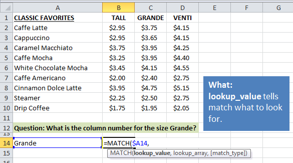
In the first argument we tell the VLOOKUP what we are looking for.  In this example we are looking for “Grande” in row 1.  I have entered the text “Grande” in cell A14, so we can make a reference to cell A14 in the formula.

2. lookup_array – This is the where argument.

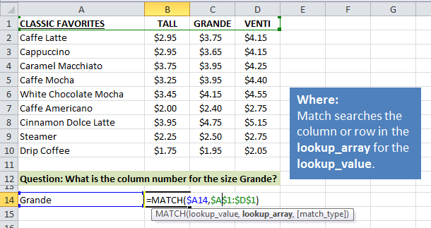
Here we need to tell MATCH where to look for the word “Grande”.  I selected the range $A$1:$D$1, which contains the column header names.  MATCH will look through row 1 from left-to-right until it finds a match.

You can also specify a column for this argument.  In that case MATCH would look down the column from top-to-bottom to find a match.

3. [match_type] – The match type tells MATCH how precise to be with the lookup.

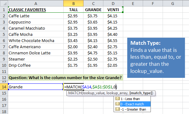
Here we specify if the function should look for an exact MATCH, or a value that is less than or greater than the lookup_value.

In this example we will use “Exact match”, which is represented by putting a 0 (zero) in the third argument.  When your MATCH is looking up text you will generally want to look for an exact match.

If you are looking up numbers with the MATCH function then the “Less than” or “Greater than” match types can be very useful.

The Result – Grande is in column 3.

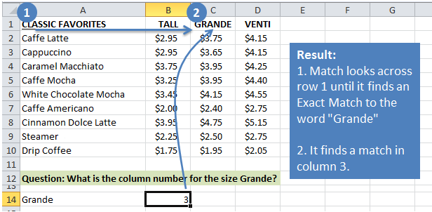
The MATCH function was able to lookup the word “Grande” in row 1 and return the value of 3 in cell B14.

Now let's see how the MATCH function can be a little more dynamic.  In the following screenshot I inserted a column to the left of column B with a new size, “Short”.

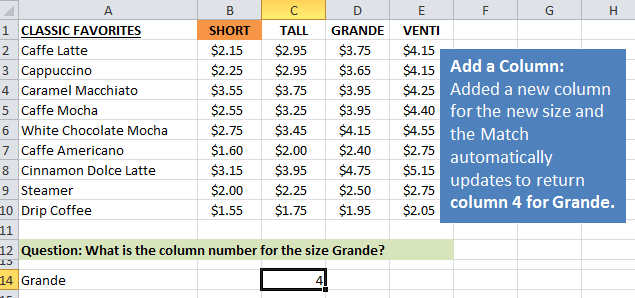
You will notice that the result of the MATCH formula changed to “4”.  This is because the word “Grande” is now in the 4th column of the lookup_array (A1:E1).

You are probably starting to see how this could help our original problem of the VLOOKUP returning the wrong result.

VLOOKUP & MATCH – The Dynamic Duo

Now let's see how we can combine these two to create a dynamic formula.

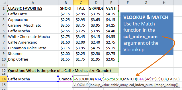
We can use the MATCH function inside the VLOOKUP function.  Instead of specifying the column number with a static number “3”, we will use the MATCH function in its place.

Since the MATCH returns a number, it is a perfect fit for the VLOOKUP's col_index_num argument.

The following example illustrates this.  You can follow along in the ‘VLOOKUP & MATCH Example' sheet in the example file.

The original formula looked like the following:

=VLOOKUP(A14,$A$2:$E$10,4,FALSE)

In the new formula I replace the “4” with the MATCH formula:

=VLOOKUP(A14,$A$2:$E$10,MATCH(B14,$A$1:$E$1,0),FALSE)

The MATCH formula references cell B14, which contains the word “Grande”.  The formula looks up the word Grande in row 1 and returns a 4 as the result because Grande is in the fourth column of the range A1:E1.

The VLOOKUP formula is now much more dynamic with MATCH included.  We can add or delete columns to the menu (table), and the VLOOKUP will still return the price for the size that is specified in cell B14.

You could also change either the item in cell A14 or the size in cell B14 to return different prices in cell C14.

This makes the formula very flexible, and easier to reuse in other places in the workbook.

Conclusion

I hope this post has helped you understand how the VLOOKUP and MATCH functions can work together to be a dynamic duo.  This team of functions will help prevent errors in your formulas.  It will also help you create financial models that are more flexible for data retrieval and scenario analysis.

Series: The Lookup Functions Explained

This is the 2nd post in a series about the most commonly used lookup functions in Excel.

1. In the first post I explained the VLOOKUP function at Starbucks.
2. In this second post I explained how to make lookup formulas more dynamic with the VLOOKUP & MATCH functions.
3. In the third post I explain the INDEX function.

Please leave a comment below with any questions or comments.

Take the VLOOKUP Challenge

I've put together 5-part video training series that will help you learn more about lookup formulas and test your skills.

Click here to take the VLOOKUP challenge