How to Create Summary Reports in Excel: Formulas vs. Pivot Tables

When your boss asks for a summary report, you want something that's easy to build and easy to update. Excel gives you several ways to do this, and each method has its trade-offs.

In this tutorial, we'll cover three approaches: a formula-based solution using UNIQUE and SUMIFS, the newer GROUPBY function, and Pivot Tables. At the end, we'll compare them so you can pick the right tool for your situation.

Download the Excel Files

Complete the form below to instantly access the Excel files and Excel Formula Prompting Guide.

Video Tutorial

Watch on YouTube & Subscribe to our Channel

Start by Converting Your Data to an Excel Table

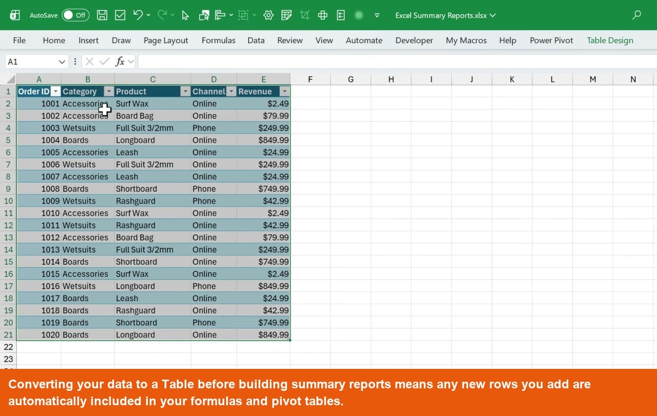
Before building any summary report, convert your data range into an Excel Table. Click any cell in your data, go to the Home tab, click Format as Table, and choose a style.

Tables give you automatic banded rows, built-in filters, and structured references that make your formulas more readable. More importantly, when you add new rows to the bottom of a table, Excel automatically extends the range. Your summary reports stay accurate without any manual adjustments.

If you are not familiar with Excel Tables yet, check out the linked video in the description. It covers everything you need to know before moving forward.

Formula Method 1: UNIQUE and SUMIFS

The first formula-based approach uses two functions together: UNIQUE to extract a distinct list of categories, and SUMIFS to calculate totals for each one.

Step 1: Get a Unique List with UNIQUE

Click an empty cell and type =UNIQUE(. The only required argument is the range you want to deduplicate. Select the Category column in your table and press Enter.

Excel returns a spill range, a dynamic list of all unique category values. If a new category appears in your source data, this list updates automatically.

Step 2: Calculate Totals with SUMIFS

In the cell next to your UNIQUE results, type =SUMIFS(. For the sum range, select the Revenue column. For the criteria range, select the Category column. For the criteria, reference the first cell of your UNIQUE spill range.

Instead of typing the cell address, select all the cells in the spill range and Excel will write H2# for you. The hash symbol tells Excel to reference the entire spill range, not just a single cell. One formula calculates totals for every category automatically.

One important note: the UNIQUE function requires Excel 2021 or later. If you or your team are on an older version, skip ahead to the Pivot Table section, which works on all versions.

Formula Method 2: The GROUPBY Function

If you are on Microsoft 365, the GROUPBY function creates the entire summary report in a single formula. No need to combine UNIQUE and SUMIFS separately.

Type =GROUPBY( and fill in three arguments: the row fields (your Category column), the values (your Revenue column), and the function, which is SUM. Press Enter.

GROUPBY returns a complete summary table with unique categories, summed revenue for each, and a grand total row at the bottom. There is also a related PIVOTBY function that adds a column fields argument, letting you break data out across multiple columns.

Build a Summary Report with a Pivot Table

Pivot Tables have been in Excel since 1994 and work on every version. They require no formulas at all. You build them with drag and drop in seconds.

How to Create a Pivot Table

1. Click any cell inside your table.
2. Go to the Insert tab and click PivotTable.
3. Choose where to place the pivot table, then click OK.
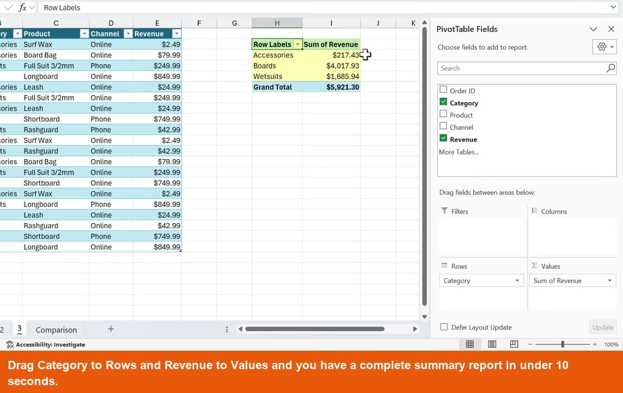
4. In the PivotTable Fields pane, drag Category to the Rows area.
5. Drag Revenue to the Values area.

Excel instantly builds a summary with unique categories, summed revenue, and a grand total row. No formulas required.

Make It Interactive with Charts and Slicers

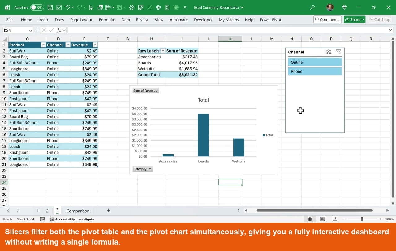
Go to the Insert tab and click PivotChart to create a chart connected directly to your pivot table. Any changes to the pivot table automatically update the chart.

Add Slicers to make your report interactive. A slicer is a visual filter. Click a slicer button to filter both the pivot table and the chart at the same time. This is how you turn a simple summary report into a full dashboard.

Formulas vs. Pivot Tables: Which Should You Use?

There is no single right answer. The best method depends on your situation. Here are the two factors that matter most.

Formatting

Formula-based results return unformatted numbers. You have to manually apply number formatting, bold the totals row, and add any color coding you want. If the data changes and rows shift, your manual formatting may end up in the wrong place.

Pivot Tables apply formatting automatically as you build them. The Design tab gives you one-click style options, and the formatting stays locked to the right rows as the data changes.

Handling New Data

When you add rows to your Excel Table, formula-based reports update automatically. New categories appear and totals recalculate without you doing anything.

Pivot Tables require a manual refresh. Right-click inside the pivot table and choose Refresh, or use the keyboard shortcut Alt+F5. If you forget this step, your report will show stale data, which can cause problems when sharing with others.

Microsoft announced an auto-refresh feature for Pivot Tables, but it was pulled from beta while they worked out some issues. In the meantime, you can set up automatic refresh with a macro if this is a recurring problem.

When to Use Each Approach

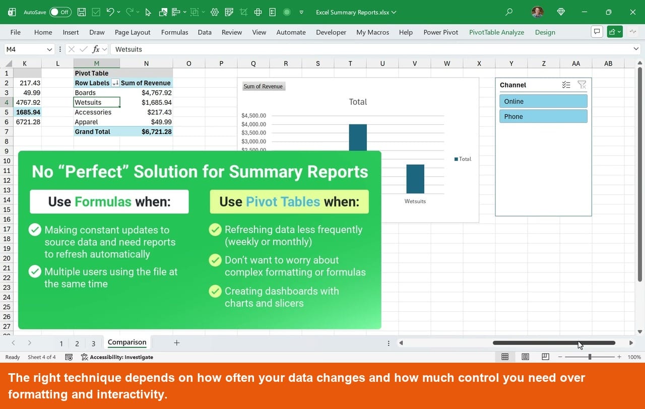
• Use UNIQUE and SUMIFS or GROUPBY when your data changes frequently or when multiple users update the source file and you need reports that always reflect the latest data automatically.
• Use Pivot Tables when data updates are infrequent (weekly or monthly), when you want to save time on formatting, or when you need interactive dashboards with charts and slicers.
• Use Pivot Tables if your team is on older versions of Excel, since UNIQUE and GROUPBY require Excel 2021 or Microsoft 365.

Which technique will you be using? Let us know in the comments below. And if you want to see more ways to automate Excel reports, check out the related videos linked in the description.