XLOOKUP has been available for over five years, and it was built to replace VLOOKUP. But a lot of people are still writing VLOOKUP formulas out of habit.
In this post we cover seven practical scenarios where XLOOKUP either simplifies your formula or does something VLOOKUP simply cannot. We also look at how Copilot can help you convert existing VLOOKUP formulas in seconds.
Download the Excel Files
Complete the form below to instantly access the Excel files and Excel Formula Prompting Guide.
Video Tutorial
Watch on YouTube & Subscribe to our Channel
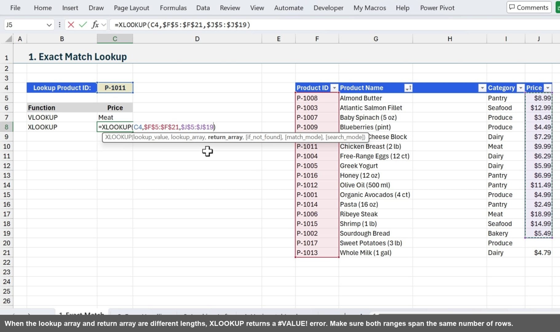
1. Exact Match Lookup
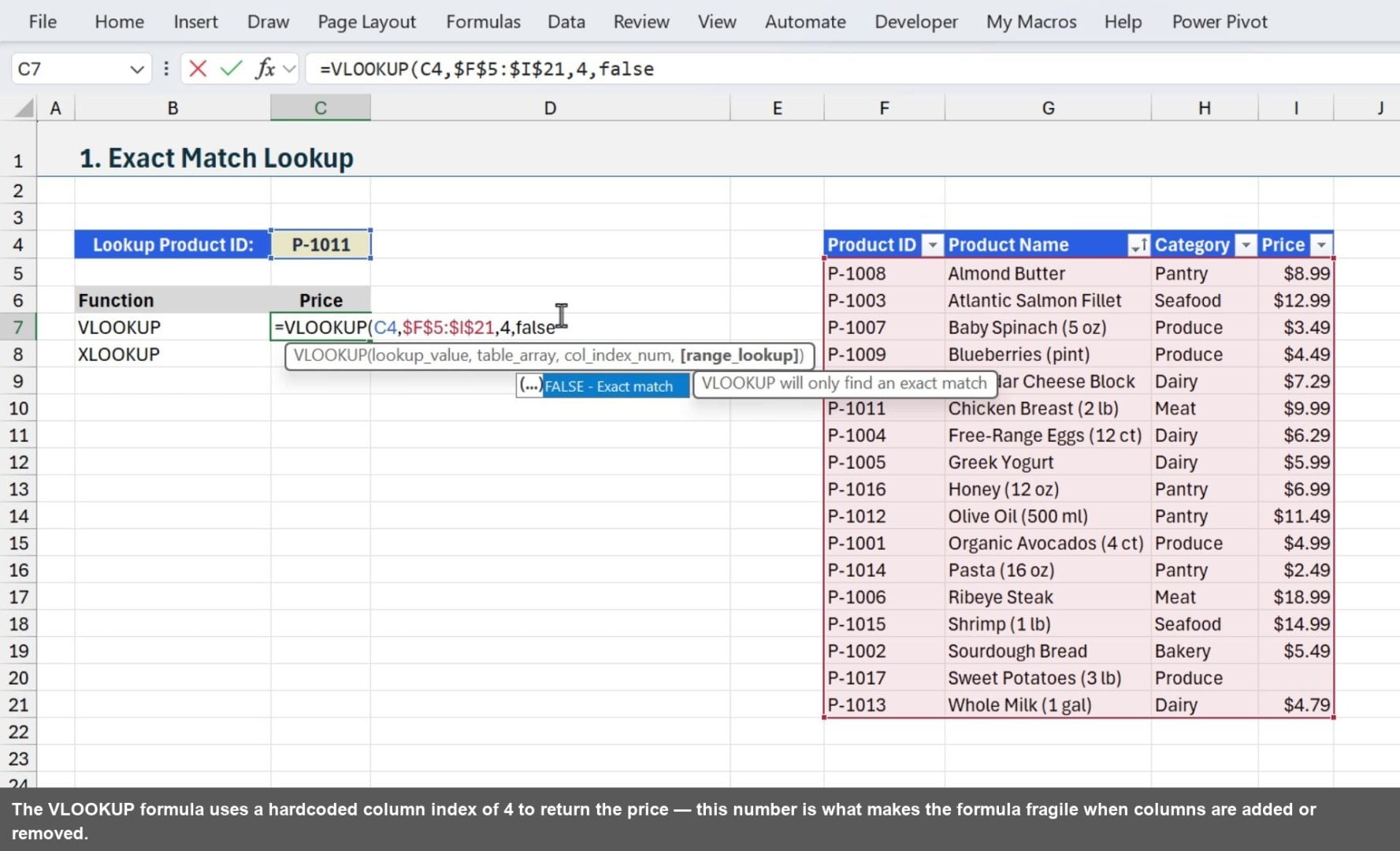
The most common lookup scenario is finding an exact match. Let's look up a Product ID and return its price from a product table.
With VLOOKUP, you select the entire table range, then specify a column index number to tell Excel which column to return.
Before diving in, a quick look at the VLOOKUP function. It searches the first column of a range for a value and returns a result from a specified column number in that range. The function arguments are:
- lookup_value: the value to search for
- table_array: the range containing both the lookup column and the return column
- col_index_num: the column number within table_array to return a value from
- range_lookup: FALSE for exact match, TRUE for approximate match (optional)
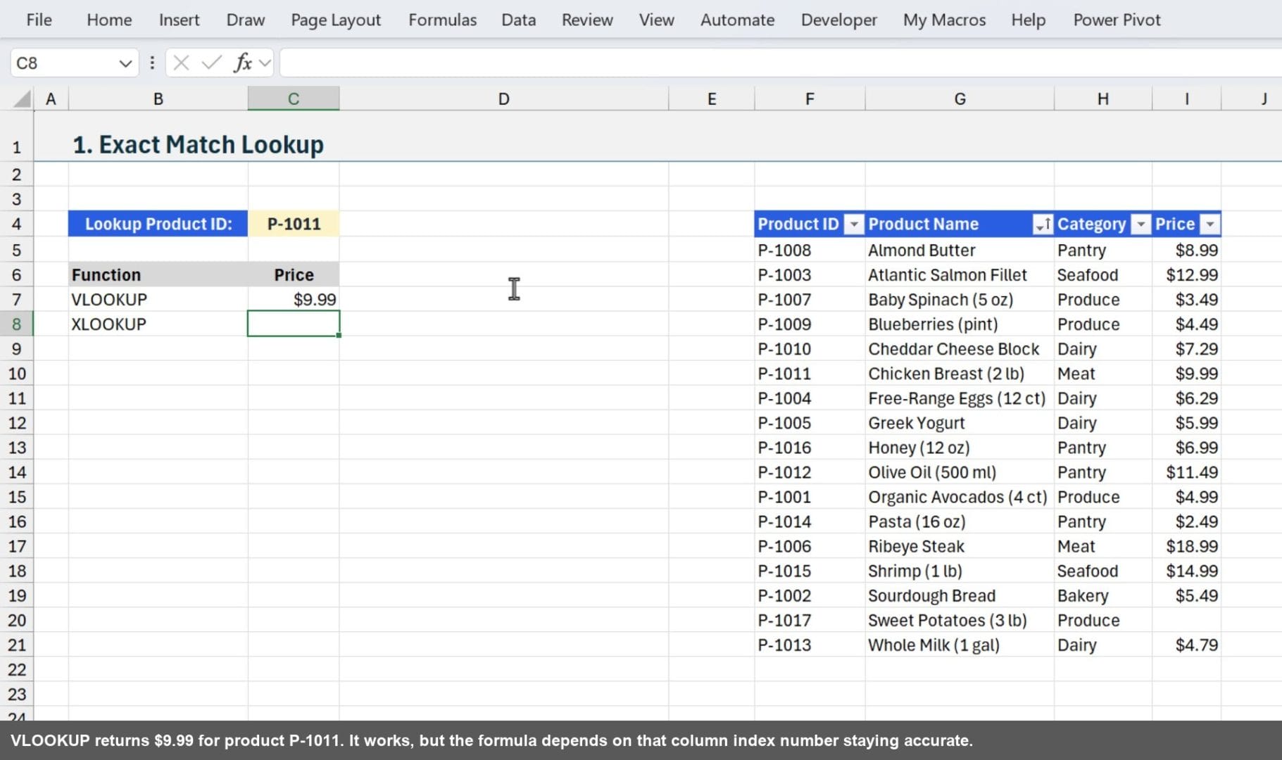
=VLOOKUP(C4,$F$5:$I$21,4,FALSE)
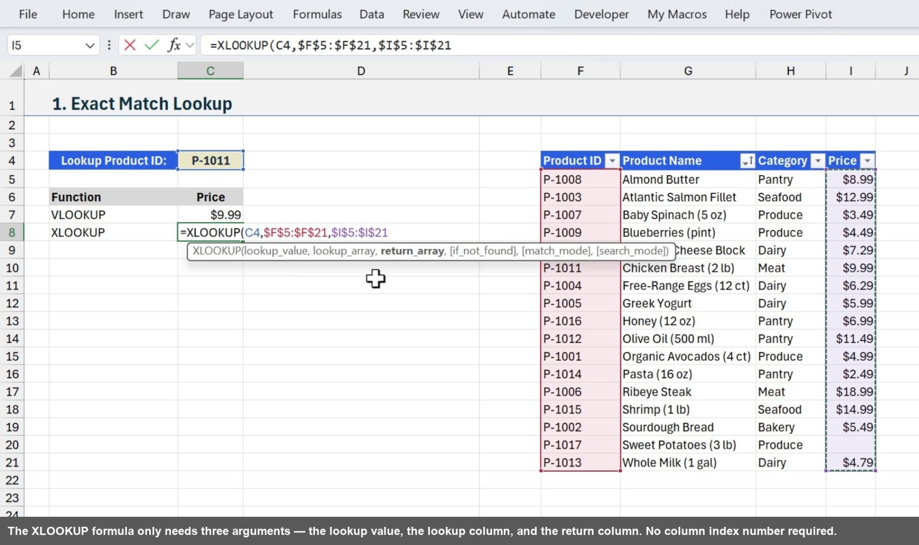
Now let's write the same lookup with XLOOKUP. Instead of selecting the whole table, you pick the lookup column and the return column separately. XLOOKUP also defaults to exact match, so there is no need to add FALSE as a fourth argument.
Here is a quick refresher on the XLOOKUP function. It searches a range or array for a match and returns a corresponding item from a second range or array. The function arguments are:
- lookup_value: the value to search for
- lookup_array: the range or array to search in
- return_array: the range or array to return a value from
- if_not_found: value to return if no match is found (optional)
- match_mode: 0 = exact match (default), -1 = exact or next smaller, 1 = exact or next larger, 2 = wildcard (optional)
- search_mode: 1 = first to last (default), -1 = last to first, 2 = binary ascending, -2 = binary descending (optional)
=XLOOKUP(C4,$F$5:$F$21,$I$5:$I$21)

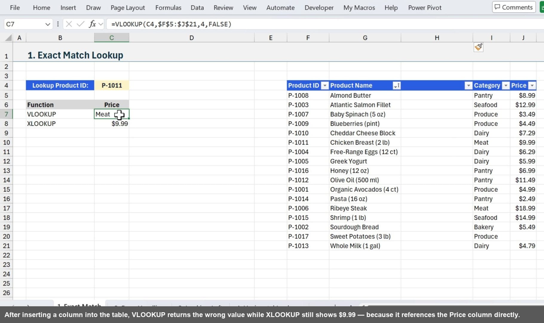
Why Separate Ranges Are Better
Because XLOOKUP references the lookup column and the return column independently, inserting a column between them does not break the formula. VLOOKUP, on the other hand, relies on a hardcoded column index number. Insert a column and that number is suddenly wrong.
Watch Out: Range Lengths Must Match
One thing to be aware of with XLOOKUP is that the lookup_array and return_array must be exactly the same length. If they are not, you will get a #VALUE! error. The easiest way to avoid this is to use Excel Tables, which automatically keep both column references the same height.
2. Error Handling
When VLOOKUP cannot find the lookup value, it returns a #N/A error. The standard fix is to wrap the formula in IFERROR.
A brief word on IFERROR. It returns a custom value when a formula produces an error, and the original result when it does not. The function arguments are:
- value: the formula or expression to evaluate
- value_if_error: the value to return if value produces an error
=IFERROR(VLOOKUP(C4,$F$5:$I$21,4,FALSE),"Not Found")
XLOOKUP handles this more cleanly. The fourth argument, if_not_found, lets you specify what to display when the lookup value is not found, with no wrapper function needed.
=XLOOKUP(C4,$F$5:$F$21,$I$5:$I$21,"Not Found")
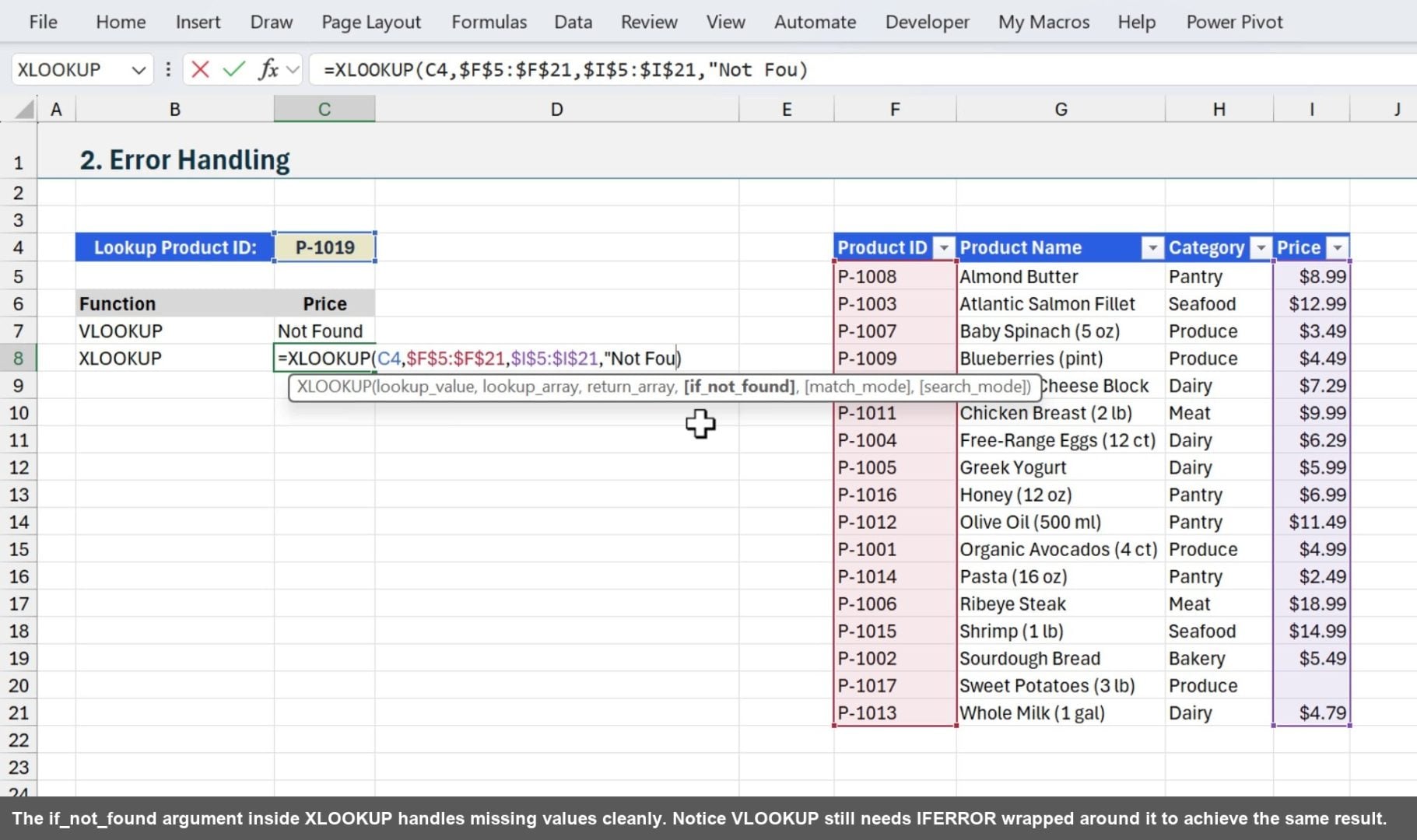
One important distinction: XLOOKUP's if_not_found only triggers when the lookup value is not found. If a different error is causing the problem (like a mismatched range length), XLOOKUP will still return that error. That is actually a good thing. It means you are not accidentally hiding real formula problems.
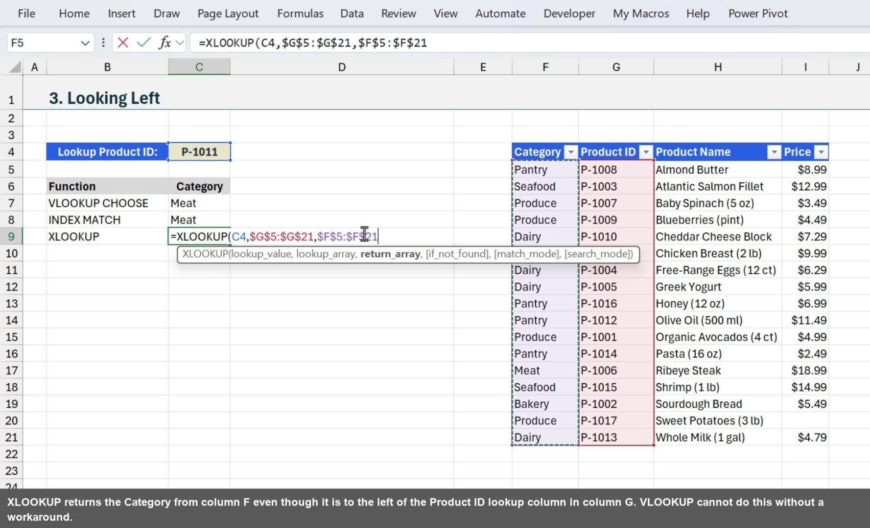
3. Looking Left
VLOOKUP can only return values to the right of the lookup column. If you need to return a value from a column to the left, you either need a CHOOSE hack or an INDEX/MATCH formula. XLOOKUP has no such restriction.
In this example the Product ID is in column G and we want to return the Category from column F, which is to the left. With XLOOKUP, we simply set the return_array to the Category column.
=XLOOKUP(C4,$G$5:$G$21,$F$5:$F$21)
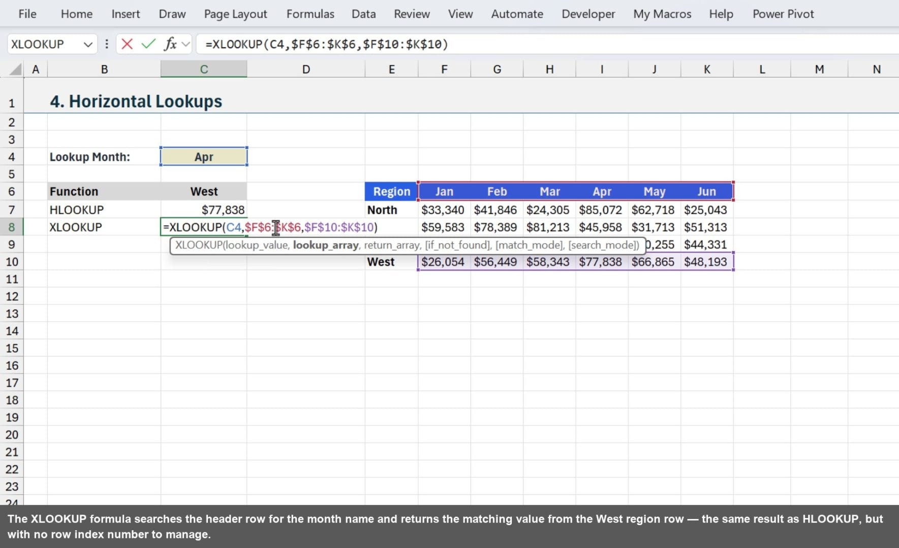
4. Horizontal Lookups
XLOOKUP replaces HLOOKUP for horizontal lookups too. Just set the lookup_array to a header row and the return_array to the data row you want to pull from. The formula structure is identical to a vertical lookup.
=XLOOKUP(C4,$F$4:$K$4,$F$7:$K$7)
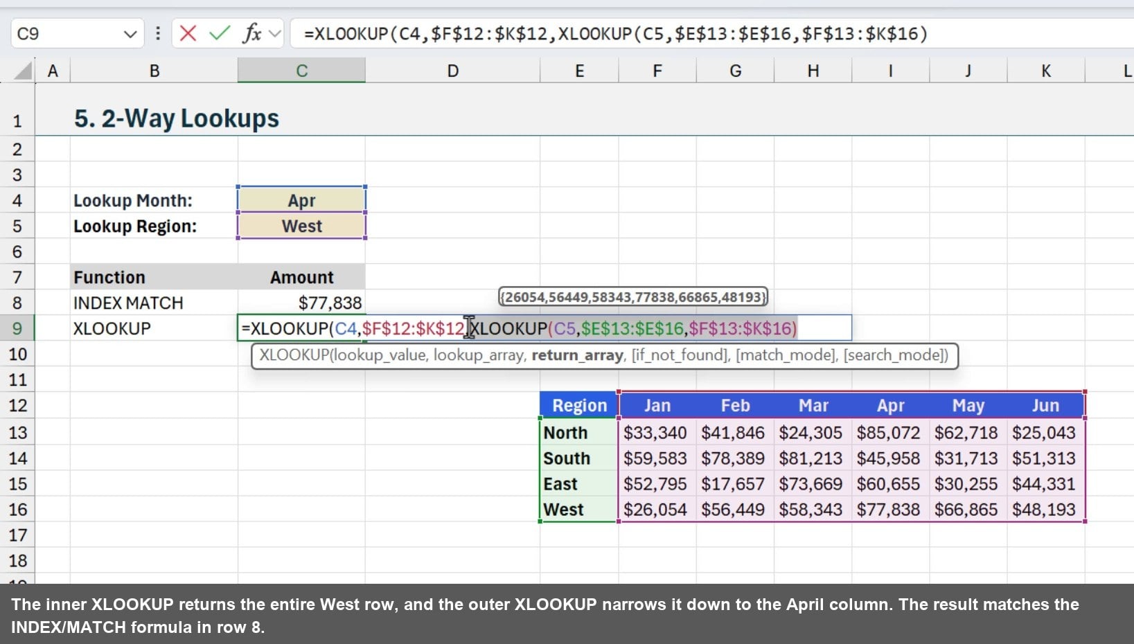
5. 2-Way Matrix Lookup with Nested XLOOKUP
To look up both a row and a column at the same time, nest two XLOOKUP formulas. The inner XLOOKUP finds the correct row of data, and the outer XLOOKUP finds the correct column within that row.
=XLOOKUP(C4,$F$12:$K$12,XLOOKUP(C5,$E$13:$E$16,$F$13:$K$16))
The inner XLOOKUP returns the entire row for the matched region. The outer XLOOKUP then finds the right column within that row. It is a clean replacement for INDEX/MATCH in a matrix lookup scenario.
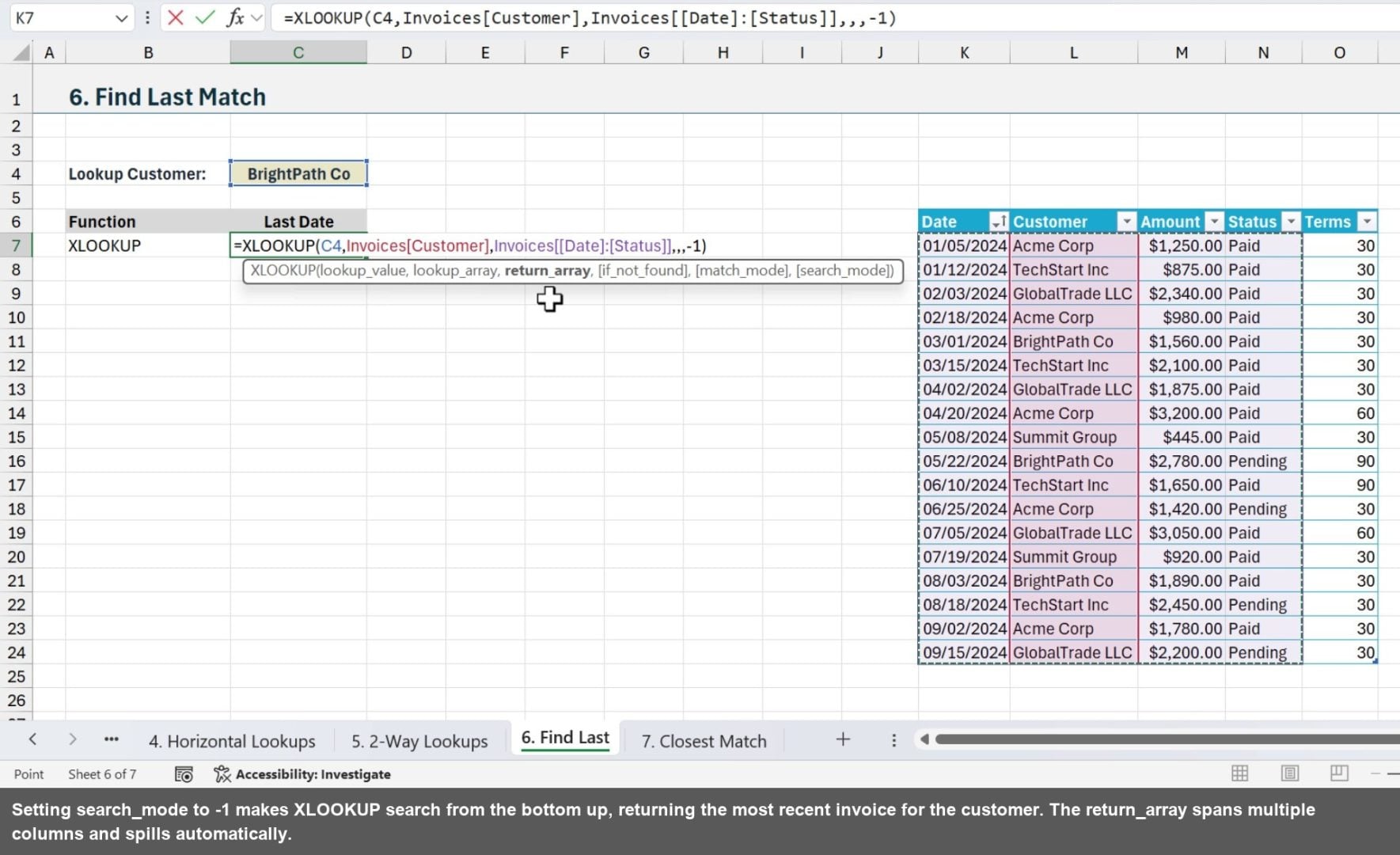
6. Find the Last Match
By default, XLOOKUP searches from top to bottom and returns the first match. Setting the search_mode argument to -1 reverses the search direction, returning the last match instead.
This is useful when you have a transaction log and need the most recent entry for a customer. You can also return multiple columns in one formula by specifying a multi-column range as the return_array.
=XLOOKUP(C4,Invoices[Customer],Invoices[[Date]:[Status]],,,−1)
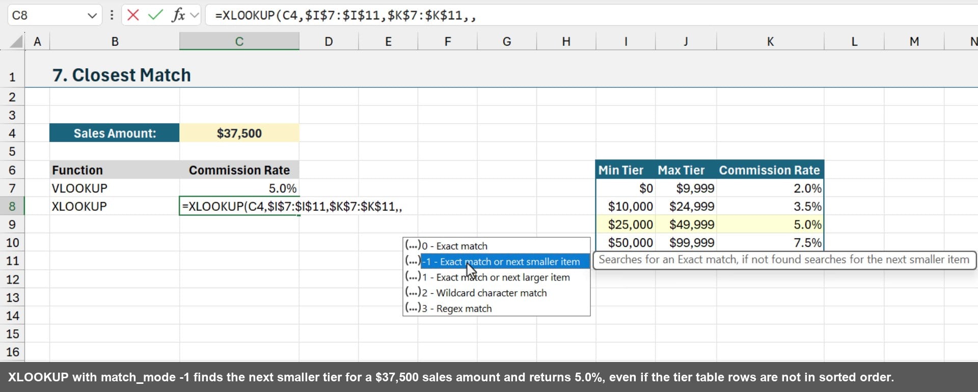
7. Closest Match Lookup
XLOOKUP can also do approximate match lookups, which is useful for tiered rate tables like commission schedules. Setting match_mode to -1 tells XLOOKUP to return the exact match or the next smaller value.
One big advantage over VLOOKUP here: XLOOKUP does not require the lookup table to be sorted. VLOOKUP's approximate match mode breaks if the data is out of order. XLOOKUP handles it correctly either way.
=XLOOKUP(C4,$I$7:$I$11,$K$7:$K$11,,−1)
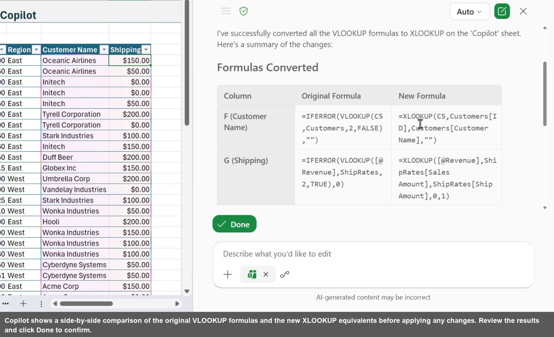
8. Use Copilot to Convert VLOOKUP to XLOOKUP
If you have a workbook full of VLOOKUP formulas, you do not have to update them one by one. Copilot in Excel can handle the conversion for you. Open the Copilot pane and describe what you want.
A prompt like this works well: “Please change the formulas on this sheet that use VLOOKUP to XLOOKUP and use the if_not_found argument within XLOOKUP instead of the IFERROR function that is wrapped around VLOOKUP.” Copilot will show you the original and updated formulas before applying the changes.
When Not to Use XLOOKUP
XLOOKUP is the right choice in almost every situation, but there is one important exception: when the people using your file are on an older version of Excel. XLOOKUP requires Excel 2021 or Microsoft 365.
Microsoft did add limited backwards compatibility for Excel 2016 and 2019, but it is view-only. Users on those versions can see the results of an XLOOKUP formula, but they cannot edit existing ones or create new ones.
If your file is shared with colleagues or clients on older Excel versions, stick with VLOOKUP or INDEX/MATCH to keep the formulas fully editable for everyone.
Summary
XLOOKUP is a genuine upgrade from VLOOKUP in almost every scenario. It is more readable, more resilient to structural changes in your data, and it replaces HLOOKUP, IFERROR-wrapped VLOOKUP, and even INDEX/MATCH in most cases.
The three required arguments are all you need for everyday lookups, and the optional arguments unlock powerful capabilities like reverse search, closest match, and multi-column returns. If you are on Excel 2021 or Microsoft 365, there is no reason to keep writing VLOOKUP.


This is so useful to know. I already use the XLOOKUP instead of VLOOKUP pretty much all the time now, thanks to the amazing Excel Campus training, and have now learned of a couple of other ways to use this formula that I wasn’t aware of. Thank you!
Thanks so much, Sheena! I’m happy to hear you have learned so much. 🙂
I agree that VileLOOKUP and HorribleLOOKUP are never the way to go, but there are a couple of additional things I would point out.
First, INDEX/XMATCH is still the best of the best because there are at least three use cases they can handle that XLOOKUP can not. Perhaps the most useful of the three cases would be simultaneously returning multiple columns (or rows) from multiple lookups. XLOOKUP can return multiple columns or rows for a single lookup or a single column or row for multiple lookups, but not both at the same time. Whereas the innate two-dimensional nature of INDEX allows it to accept multiple row_num and column_num values simultaneously. In other words, a single spillable INDEX/XMATCH can return multiple rows and columns of results at once.
=INDEX(from_this_range,XMATCH(find_these_values,in_this_column),XMATCH(and_these_headers,in_this_row))
Second, IFNA is a better option than IFERROR when it comes to failed lookups because a failed lookup will only ever return #N/A, whereas IFERROR is a sledge hammer that will react to literally any error. For example, hasty typing could result in a misspelled formula: =IFERROR(INDEXreturn_from,XMACTH(find,by_searching)),”match not found”)
Since XMATCH is misspelled, the correct result should be the #NAME? error, but IFERROR will intercept that and treat it the same as an #N/A so that the result would be “match not found” when in fact the lookup was never even attempted.
Great points, David! I’ll do a follow-up on more advanced use cases.