Bottom line: Learn how to use the VLOOKUP function to find the closest match by setting the last argument to TRUE.
Skill level: Intermediate
Do you have a common activity you do when you stay home sick from work or school? For me, it always included watching an episode of The Price is Right with Bob Barker.
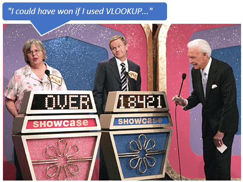
If you have never seen it, The Price is Right is a game show in the U.S. where contestants have to guess the prices of various household items. For the Showcase game, the contestant must guess a price that is equal to or less than the actual retail price of the items to win the game.
If the contestant could use a vlookup formula to make their guess, they would win every time! The contestant would have to set the last argument in the vlookup to TRUE for this to work.
When you start using vlookup you typically set the last arguement [range lookup] to FALSE. This tells vlookup to find an exact match for the text or number you are looking for. Checkout my article on VLOOKUP Explained at Starbucks for more info.
Closest Match with VLOOKUP (TRUE)
Setting the last argument to TRUE tells VLOOKUP to find the closest match to the text or number you are looking for. However, there is a caveat to this “closest match”…
The VLOOKUP starts at the top of the range you specify and looks down (vertically) in each cell to find the value you are looking for (lookup value). It stops searching when it finds a value that is greater than or equal to the lookup value.
In the screencast above the vlookup formula is looking for the number 14 in the list. Since 14 is not in the list, it returns 10. But why???
Well, there are three possible outcomes for vlookup when the last argument is TRUE. The results may seem confusing at first, but they can actually be quite useful.
You can download the file to follow along.
Outcome #1: VLOOKUP Finds Exact Match
If vlookup finds a value that is equal to the lookup value then it returns a result from that same row.
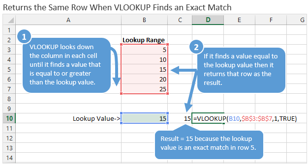
This is essentially the same as a normal vlookup where you set the last argument to FALSE. The function finds an exact match and returns that row as a result.
Outcome #2: VLOOKUP Finds Closest Match
If vlookup finds a value that is greater than the lookup value, then it returns a result from the previous row.
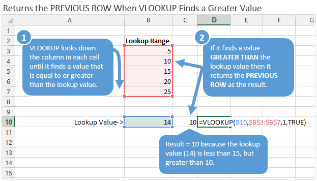
This means that the “closest match” is going to be less than or equal to the lookup value.
It's also important to note that if the lookup value is greater than the last cell in the lookup range, then the result will be the value in the last cell.
For example, if the lookup value was 30 in the example above, vlookup would return cell B7 (25) as the result. Since vlookup has no more values to look at, it stops at the last cell.
Outcome #3: VLOOKUP Returns an #N/A Error
If vlookup finds a value that is less than the first cell in the lookup range, then it returns an error.
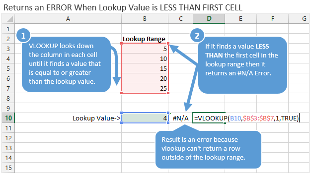
We probably spend a lot of time figuring out why vlookup formulas are not working, and returning errors. This is no exception when using vlookup to find the closest match.
If you are looking up numbers, then the first row in the lookup range needs to be the minimum amount you will potentially lookup. I explain more about this in the example below.
Important: Sort the Lookup Range
Most of the time you will want the numbers in the first column of the lookup range sorted from smallest to largest (A-Z).
The “V” in VLOOKUP stands for vertical. As I explained above, it starts at the top cell in the lookup range and works its way down. As soon as it finds a cell greater than or equal to the lookup value, IT STOPS!
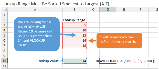
So if you have values at the bottom of the list that are smaller, vlookup will never find them.
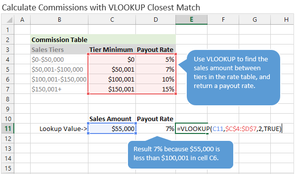
Example: Calculating Commissions with VLOOKUP
One of the best examples of this technique is calculating commissions. Please see my article on calculating commissions with vlookup for a full explanation on this technique.
Click here to read the full article on calculating commissions
The Price is Right for VLOOKUP's Closest Match
So this is why it would be great for The Price is Right contestants to have a vlookup at their disposal. If they try to guess a price that is too high, vlookup would return the closest match that is equal to the actual retail price. I know it's a stretch, but think about it next time your writing a vlookup formula. 🙂
The host of the show, Bob Barker, always used to have the same closing statement at the end of the show about getting your pets neutered. I think he had something against puppies and kittens… j/k
In closing this post, I will remind you to always sort the first column in your lookup range when finding the closest match with vlookup.
Please leave a comment below with any questions. Thanks!


Actually, all these vlookup tutorials were really helpful to me. I am working in a manufacturing company & advanced excel knowledge is far more important to work with complex reports to me and therefore, I wanted to find a source to learn excel more.When i was searching on net i could find your free excel tutorials and after that i registered with your site now i know considerable things about excel vlookup,pivot table, and some more.And also,I must be grateful to you for your valuable support for worldwide people who really have a thirst to learn excel.Finally, I wish you all the best for your campaign and I need to refer your tutorials further to sharpen my excel knowledge.
Thank you,
Damith Jayaruwan.
Thank you for the kind words Damith! I’m happy to hear that you are learning Excel and enjoying the tutorials. Thanks for subscribing to the newsletter as well. Have a great day! 🙂
You are so succinct in how you explained the closest match! You have explained it better than other websites I have visited. You have the gift!
Dear Jon,
Hi
thankfully for you because learn excel tips and vba.
[…] How to Use VLOOKUP to Find the Closest Match (TRUE) post by Jon Acampora […]
Wonderfully explained.
Thanks Anas!
You make excel functions seem simple!
Thank you.
Thank you Maria! 🙂
I am interested in finding literally the closest number. In your examples above when you search for 14, it returns 10 which is next lower number. But 14 is closer to 15 than it is to 10 so how can I get Excel to return “15” when I go into the table with a lookup value of 14? (Or is that what the “False” parameter does?)
Thanks,
Chip
Hi Chip,
Great question! You can use an array formula for that. Here is an article with an example. I hope that helps.
here’s a way to find the the next number in sequence that’s equal to or greater than the search-value. Assume 4 is the search-value, and $A$1:$A$10 is the search-range. Should be entered as an array formula (CTRL-SHIFT-ENTER):
=MIN(IF($A$1:$A$10 >= 4, $A$1:$A$10, “”))
Thanks for the suggestion John! We can also use the MATCH function and set the [match_type] parameter to -1 to find a value greater than the search value. This avoids the need for an array formula. So many ways to accomplish a task in Excel. I guess that’s what makes it fun. 🙂
Dear Jon,
I still fail to understand that why would we at all be looking for a closest match, when the cell is filled with an exact match.
Can you please throw some light.
Thanks in advance
Sunil
Dead simple explanation, thank you!
Of course, with me, this results in a new question: will this work with times, rather duration, as well? Reason I ask is that I’m part of a running club and one of the runners suggested we should guess all our groups participants for the next half marathon.
I’d love to be able to create a sheet where the runners can fill in their estimate for all their fellow runners and have the sheet show who was the closest to the actual times they ran.
Thanks Phil! 🙂 Yes, it can work for times. Times are just decimal numbers in Excel that are formatted as a time. Check out my article on how dates work in Excel for more info. I also have an article on 3 ways to Group Times that you might be interested.
Hi John,
How would I go about using the excel lookup for commission when the tiers are I different groups. For example let’s say there are 2 groups (so 2 tables) you fall under depending on your job title. So I have 4 categories and 3 of them are in Group A and one is in group B. How would I make the calculations so they know which table to pull from?
Hi Indira,
Great question! You can use the IF or CHOOSE function to first determine what group they are in, then use the vlookup based on the group. The basic outline of the formula would look like the following.
=IF(A2=”Group A”, Vlookup(),Vlookup())
If there are more than two groups then you can use the CHOOSE function. I cover this in more detail in my Ultimate Lookup Formulas Course.
I hope that helps. 🙂
Jon,
I feel like I’m missing something here. Where “Outcome #1: VLOOKUP Finds Exact Match” says:
“This is essentially the same as a normal vlookup where you set the last argument to FALSE. The function finds an exact match and returns that row as a result.”
The example has code with last argument value “True” and not “False”. Is the example right? If it is, perhaps I need to spend more time ingesting it.
Great article!
Love the “Closest Match” moving illustration!!!
– Deborah
Hi Deborah,
In that first outcome, if the lookup value exists in the table_array then the Vlookup will return the row of the matching value. This is the same behavior as if the last argument were set to FALSE. In that sentence I was just trying to say that it is the same behavior as if the last argument were set to FALSE. The argument is still set to TRUE for this example. Sorry if that was confusing.
Hi Jon,
I’m trying to do a vlookup where I’m using an address say 115 King Street South as my lookup_value, but in the table_array the address may be more like 115 KING ST S. I want it to pull the associated available space (5,236 SF). I think the vlookup is missing the address because it is not exactly the same.
Is there a solution for this?
Thank you,
Jessica
Hi, i am trying to make a report. For login time for employees… Problem with raw data is that it randomly throws 2 to 3 instance of of same employee with diffrent login time . So i have to manually pick the nearest login time to a reference… Example.( Suppose my shift starts from 9:00 am but in report it gives my name in the list 3 times. And it gives 3 diffrent time (say) 9:12am 8:58 am and 9:20am . The value i have to pick is 8:58 am which is nearest to 9:00 am. So is there any combinatiojnof formula or any helper columnbi can add to acheive this vlookuo
Woooooaaaaahhhh! I’ve been trying to use Vlookup for ages to retrieve a value based upon a date. Your top animation explained it to me in a way I understand. Thanks so much!
Great article!
Can this work for finding the closest Match “TEXT”? I tried, but it does not work. Is there another formula to do this?
Use VBA
Hey John,
Nice article. I ma struggling with finding the pair with least mean scores. Can you help in this regard.
the data looks like:
Race: B black, W white
Race Mean
B1 3.5964
B2 4.3333
B3 4.0467
B4 4.3567
B5 4.0760
W1 4.3918
W2 4.4152
W3 3.5438
W4 4.5847
W4 3.8771
I am trying to calculate Pairs with smallest difference based on mean scores. Can you please guid me through it.
thanks,
Regards,
Naeem
Hi Jon,
THANK YOU SO MUCH for the explanation. So clear and didactic.
I was going nuts for a while trying to figure out based on what vlookup decides to return values when these are not an exact match.
Now it is clear to me.
Thanks again!
Thank so much for the nice feedback Joseph! I’m happy to hear it helped. 🙂
Thanks for the reminder, much appreciatedf
Thanks for the reminder, much appreciated.
In Example No1 where it states ‘Find the Closest match’ 15 is closer to 14 than 10 is so why is 10 deemed to be the closest match? It makes no sense.
How do I get 15 as the answer (as it is only 1 away from 14) and NOT 10 (which is 4 away from 14?
Hi there I’d like to find
I have a list of sizes S,M,L and widths S=50 M =100 and L=200
I would like to test my width is greater than sizes and return options available for example
width of 30 would return S,M,L
width of 90 would return M,L
width of 190 would return M,L
width larger would return “message”
I get equal value or grater than value how
Non-array formula for closest value (above or below) in ascending-sorted list (using example from above article):
=IFERROR(INDEX(B3:B7,MIN(COUNT(B3:B7),MATCH(B10,B3:B7,1)+B10>AVERAGE(OFFSET(INDEX(B3:B7,MATCH(B10,B3:B7,1)),,,2))))),B3)
OFFSET() finds BOTH the closest value above AND below.
AVERAGE() finds the mid point between the closest value above and below.
IFERROR() resolves for values below the lowest value in the list.
MIN()/COUNT() resolves for values above the highest value in the list.
I have not seen a similar method in my online search.
Formula should read…
=IFERROR(INDEX(B3:B7,MIN(COUNT(B3:B7),MATCH(B10,B3:B7,1)+(B10>AVERAGE(OFFSET(INDEX(B3:B7,MATCH(B10,B3:B7,1)),,,2))))),B3)
GENIUS!
Great article! Big thumb up!
Last minute here: Simple Question. Can i add a V lookup into the middle of an existing formula? I have 12 data sets. 2 of which are currency. I need them to redirect to a point system. SO: $10,000 = 200, $20,000 = 400 but $25,000 still=400. Only $10,000 increments warrant that 200 point. Same for next column. 1000=100 2000=200 2500=200 still.
Posting current Equation. Would I be able to vLookup for column F3 & H3?
=(B3/AC$4)*AD$4+(D3/AC$5)*AD$5+(F3/AC$6)*AD$6+(H3/’YTD (2)’!AC$17)*AD$17+(J3/AC$32)*AD$32+(L3/AC$33)*AD$33+(N3/AC$34)*AD$34+((P3>1)*100)+(R3/AC$36)*AD$36+(T3/AC$37)*AD$37+(V3/AC$38)*AD$38
I have a list of values sorted in a column like this:
8.5
23.5
32.0
38.0
46.5
61.5
70.0
Say my search value is 10.
How can I get Excel/Sheets to find the value equal to or greater than 10? In this case I want the value 23.5.
Your training videos are great… but I am looking for a formula that will run like the Vlookup but will select all the matches instead of stopping at the first one. I’m very new at learning the more complex of formulas.
No questions, just wanted to say that I LOL’d at the Price Is Right example at the beginning of this post. Thanks for explaining how TRUE works in the range_lookup.
Hi, Is there a way to find one of the strings in the named range using VLOOKUP. For some reason, this does not work with a named range but works without a named range.
Great post! Using VLOOKUP with the closest match is a game changer for my data analysis tasks. I appreciate the clear examples you provided, they made it much easier to understand how to implement this in my own spreadsheets. Thank you for sharing!