Bottom line: Learn 3 tips for writing and creating formulas in your VBA macros with this article and video.
Skill level: Intermediate
Video Tutorial
Download the File
Download the Excel file to follow along with the video.
Automate Formula Writing
Writing formulas can be one of the most time consuming parts of your weekly or monthly Excel task. If you're working on automating that process with a macro, then you can have VBA write the formula and input it into the cells for you.
Writing formulas in VBA can be a bit tricky at first, so here are 3 tips to help save time and make the process easier.
Tip #1: The Formula Property
The Formula property is a member of the Range object in VBA. We can use it to set/create a formula for a single cell or range of cells.
There are a few requirements for the value of the formula that we set with the Formula property:
- The formula is a string of text that is wrapped in quotation marks. The value of the formula must start and end in quotation marks.
- The formula string must start with an equal sign = after the first quotation mark.
Here is a simple example of a formula in a macro.
Sub Formula_Property()

  'Formula is a string of text wrapped in quotation marks
  'Starts with an = sign
  Range("B10").Formula = "=SUM(B4:B9)"

End Sub
The Formula property can also be used to read an existing formula in a cell.
Tip #2: Use the Macro Recorder
When your formulas are more complex or contain special characters, they can be more challenging to write in VBA. Fortunately we can use the macro recorder to create the code for us.
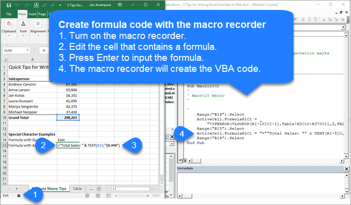
Here are the steps to creating the formula property code with the macro recorder.
- Turn on the macro recorder (Developer tab > Record Macro)
- Type your formula or edit an existing formula.
- Press Enter to enter the formula.
- The code is created in the macro.
If your formula contains quotation marks or ampersand symbols, the macro recorder will account for this. It creates all the sub-strings and wraps everything in quotes properly. Here is an example.
Sub Macro10()
'Use the macro recorder to create code for complex formulas with
'special characters and relative references

  ActiveCell.FormulaR1C1 = "=""Total Sales: "" & TEXT(R[-5]C,""$#,###"")"

End Sub
Tip #3: R1C1 Style Formula Notation
If you use the macro recorder for formulas, you will notices that it creates code with the FormulaR1C1 property.
R1C1 style notation allows us to create both relative (A1), absolute ($A$1), and mixed ($A1, A$1) references in our macro code.
R1C1 stands for Rows and Columns.
Relative References
For relative references we specify the number of rows and columns we want to offset from the cell that the formula is in. The number of rows and columns are referenced in square brackets.
The following would create a reference to a cell that is 3 rows above and 2 rows to the right of the cell that contains the formula.
R[-3]C[2]
Negative numbers go up rows and columns to the left.
Positive numbers go down rows and columns to the right.
Absolute References
We can also use R1C1 notation for absolute references. This would typically look like $A$2.
For absolute references we do NOT use the square brackets. The following would create a direct reference to cell $A$2, row 2 column 1
R2C1
Mixed References
with mixed references we add the square brackets for either the row or column reference, and no brackets for the other reference. The following formula in cell B2 would create this reference to A$2, where the row is absolute and the column is relative.
R2C[-1]
When creating mixed references, the relative row or column number will depend on what cell the formula is in.
It's easiest to just use the macro recorder to figure these out.
FormulaR1C1 Property versus Formula Property
The FormulaR1C1 property reads the R1C1 notation and creates the proper references in the cells. If you use the regular Formula property with R1C1 notation, then VBA will attempt to put those letters in the formula, and it will likely result in a formula error.
Therefore, use the Formula property when your code contains cell references ($A$1), the FormulaR1C1 property when you need relative references that are applied to multiple cells or dependent on where the formula is entered.
If your spreadsheet changes based on conditions outside your control, like new columns or rows of data are imported from the data source, then relative references and R1C1 style notation will probably be best.
I hope those tips help. Please leave a comment below with questions or suggestions.


Hi Jon!
Is it possible to make that construction dynamic? I mean the SUM function
Sub LastCell_Total ()
Dim lCell as Range
Set lCell = Range(“I2”).End(xlDown).Offset(1, 0)
lCell.Formula = WorksheetFunction.Sum(Range(Range(“I2”), Range(“I2”).End(xlDown)))
End Sub
Hi Claudiu,
Great question! Yes, absolutely.
You could declare a variable to hold the last row number. Or use the Row property of lCell.
Then use the variable in the formula string. Concatenate it with the ampersands. Here is an example.
Range(“A4”).Formula = “=SUM(B4:B” & lCell.Row & “)”
When that evaluates is will create the range reference with the last row number after B. Something like B4:B203
I hope that helps.
Hi Jon,
first of all, Thank You for your answer. In my example, “lCell” is the place where I need the Sum function. And the Sum function should add the values from column I2 to I
Can you help me to understand and resolve that?
Thank you again
The FormulaR1C1 property reads the R1C1 notation and creates the proper references in the cells. If you use the regular Formula property with R1C1 notation, then VBA will attempt to put those letters in the formula, and it will likely result in a formula error.
Hi Jon,
Can you please explain on what you say on the top?
You are saying same thing but one creates error and one not!
Regards,
G
Hi G,
If you are using R1C1 style notation in your formula text, then it is best to use the FormulaR1C1 property.
Notice how this line uses FormulaR1C1
Range(“B3:B12”).FormulaR1C1 = “=RC[1]+RC[2]”
The following line uses R1C1, but uses the Formula property.
Range(“B3:B12”).Formula = “=RC[1]+RC[2]”
That line could result in an error if you have mixed references. Most of the time VBA will figure it out and still convert the R1C1 to cell references. As the formula gets more complex then it might not be able to convert it. Therefore, it’s best to use FormulaR1C1 when you have R1C1 references in your formula text.
I hope that helps.
Hello Jon,
How can we run macro for a range of cells instead of one cell?
-We want to copy all formula for not only B3, but B3:B12. How can we do that?
Regards,
G
Hi G,
When using R1C1 style notation you can apply the same formula to all the cells in a range. Here is an example.
Range("B3:B12").FormulaR1C1 = "=RC[1]+RC[2]"That line of code would put the same formula in each cell. The formula in cell B3 would evaluate to C3+D3. The formula in cell B4 would be C4+D4.
If you already have a formula in cell B3, then you can just copy it down to the rest of the cells. There are many ways to do this, but here is one simple line of code using the Copy method.
Range("B3").Copy Range("B4:B12") Checkout my article on 3 Ways to Copy and Paste Cells with VBA Macros + Video for more details on these techniques.Hi Jon,
Let’s make this more complicated…
My formula is an array formula that needs to have named ranges changed when I create a new sheet. For example, the I need is an array formula that contains a range that is named data6. When I create the new month, I need to rename data6 to data7. I have been doing this manually each month, but there are 7 cells, each with different formulas that need to be changed.
Example of my working formula in Excel:
{=IFERROR(INDEX(data2,MATCH(1,(pNum2=B4)*(action2=”Retain”),0),12),”n/a”)}
Failed VBA attempts: Earlier code has already set monNum to the number of the current month. rng1 is dim as String. I’m sure it has to do with how I’m referring to the named ranges, but stumped as to how to do it.
1. Range(“L3”).Select
Selection.FormulaArray = _
“=IFERROR(INDEX(data” & monNum,MATCH(1,(pNum5=RC2)*(action5=””Retain””),0),12),””no test””)”
Returns expected end of statement
2. Range(“L3”).Select
Selection.FormulaArray = _
“=IFERROR(INDEX(rng1,MATCH(1,(pNum5=RC2)*(action5=””Retain””),0),12),””no test””)”
returns {=IFERROR(INDEX(RNG1,MATCH(1,(pNum5=RC2)*(action5=”Retain”),0),12),”no test”)}
Hi Barbara,
You are on the right track here. The variables will NOT be wrapped in quotes since they are evaluated in the VB Editor. However, the rest of the formula does need to be wrapped in quotes.
The variables and strings are joined together with ampersands. Here is an example where rng1 is a variable that is declared and set in the macro.
“=SUM(” & rng1 & “)”
Notice that after the variable we have another ampersand and then text wrapped in quotes.
This same technique will apply to your formula. Join the text after the variable with an ampersand and quotes.
I hope that helps. Thanks! 🙂
Hi Jon
Thank you for giving the simple examples and not just focused on the question asked because I was able to use the & and variable reference to put a value that was in one worksheet into another and my formula worked finally.
Using this helped me resolve an issue where I was trying to use VBA to put the contents of one cell on one sheet into another sheet. No matter what i did I kept getting Error 424 (Object required)
I was using this code:
Set CSheet =”CountCodes”
Set PSheet =”MainSheet”
Worksheets(CSheet).Range(“C13”).value = Worksheets(PSheet).Range(“C13”).Value
I solved it with your help with the following:
Sheets(CSheet).Activate
Range(“C13”).Select
Selection.FormulaR1C1 = “=” & PSheet & “!RC”
So simple. Thank you so much. It was driving me nuts.
Hi Jon…
15 years ago I used Clipper (under DOS) program, and now I’m learn Macro.
Can U help me to make it in Macro for this code :
‘( This is to make 10 variable from var1, var2… var_n with its value = “YES”)
‘——————————–
i = 1
do while i <= 10
n = alltrim(str(i))
var&n = "YES"
i = i + 1
endd
'———————————
The result from this code : var1="YES" , var2="YES" ……var10="YES"
Please email to [email protected]
Thx for your Help
Regards
Agus Gunawan
Thanks for sharing your thoughts about meta_keyword. Regards
Hi Jon,
Is there an advantage or disadvantage to using:
Range(“B10”).Formula = “=SUM(B4:B9)”
vs
Range(“B10”).Value = “=SUM(B4:B9)”
Thanks,
Mickael
Hi Mickael,
Those two lines are going to produce the same result. The major difference between the Range.Formula and Range.Value properties is when we use them to Read values back into VBA. If we want to get/return the formula in a cell then we can use the Formula property. The Value property will return the result of the formula that is displayed in the cell.
When we are using Formula or Value to write the string to the cell, then the results will usually be the same. I say “usually” because I’m not 100% sure that the results will always be the same. I think those would be rare cases with number formatting if there were differences.
I like to use the Formula property just to make the code easier to read and/or search, but that is mostly personal preference. I hope that helps.
Hi Jon,
I have below value in cell and i want to calculate that value in the next column, could you please help me??
Value==> “OG (08:30-18:00)” ==> “9:30”
I want compute time inside bracket and the output should be total time(9:30).
Thanks and Regards,
Vishal
Hello Jon
Can you help me. I am new in this area. I need to make a macro that calculates the no of empty cells in a coulmn and return the number in the first empty cell. I have so far managed to come up with:
Sub Macro2()
Range(“A2”).End(xlDown).Offset(1, 0).Select
ActiveCell.FormulaR1C1 = “=COUNTBLANK(R[-10]C:R[-1]C)”
End Sub
My problem is that I always want the formula range to end with R[-1]C but I also want it to start with A2. Is there a way to do this.
Best Regards
Louise
Hi!
Can we create a formula that divides cell that is dynamic depending on where the active cell is located?
Sample:
= /
Hi Jon,
I’ve tried the 3 tips you gave but none of them is working.
I think my formula might be too long and that is why I’m allways receiving a runtime error 1004.Can you please advice me ?
Thank you.
best regards.
Formula
=IF(B2=””;””;IF(OR($L2=1;AND(OR($M2=7;$M2=8;$M2=20;$M2=21;$M2=22);OR($L2=1;$L2=2;$L2=3;$L2=4;$L2=5;$L2=6;$L2=7));AND($L2=7;OR($M2=12;$M2=13;$M2=14;$M2=15;$M2=16)));”Other moments”;IF(AND(OR($L2=2;$L2=3;$L2=4;$L2=5;$L2=6);OR($M2=9;$M2=10;$M2=11;$M2=12));”All days 9h-13h”;IF(AND(OR($L2=2;$L2=3;$L2=4;$L2=5;$L2=6);OR($M2=13;$M2=14;$M2=15;$M2=16));”All days 13h-17h”;IF(AND(OR($L2=2;$L2=3;$L2=4;$L2=6;$L2=7);$M2=17);”All days exc Thursday 17h-18h”;IF(AND(OR($L2=2;$L2=3;$L2=4;$L2=6;$L2=7);$M2=18);”All days exc Thursday 18h-19h”;IF(AND(OR($L2=2;$L2=3;$L2=4;$L2=6;$L2=7);$M2=19);”All days exc Thursday 19h-20h”;IF(AND($L2=5;$M2=17);”Thursday 17h-18h”;IF(AND($L2=5;$M2=18);”Thursday 18h-19h”;IF(AND($L2=5;$M2=19);”Thursday 19h-20h”;”Saturday morning”))))))))))
Tip 1
ActiveCell.FormulaR1C1 = _
“IF(OR($L2=1;AND(OR($M2=7;$M2=8;$M2=20;$M2=21;$M2=22);OR($L2=1;$L2=2;$L2=3;$L2=4;$L2=5;$L2=6;$L2=7));AND($L2=7;OR($M2=12;$M2=13;$M2=14;$M2=15;$M2=16)));””Other moments””;IF(AND(OR($L2=2;$L2=3;$L2=4;$L2=5;$L2=6);OR($M2=9;$M2=10;$M2=11;$M2=12));””All days 9h-13h””;IF(AND(OR($L2=2;$L2=3;$L2=4;$L2=5;$L2=6);OR($M2=13;$M2=14;$M2=15;$M2=16));””All days 13h-17h””;IF(AND(OR($” & _
“=3;$L2=4;$L2=6;$L2=7);$M2=17);””All days exc Thursday 17h-18h””;IF(AND(OR($L2=2;$L2=3;$L2=4;$L2=6;$L2=7);$M2=18);””All days exc Thursday 18h-19h””;IF(AND(OR($L2=2;$L2=3;$L2=4;$L2=6;$L2=7);$M2=19);””All days exc Thursday 19h-20h””;IF(AND($L2=5;$M2=17);””Thursday 17h-18h””;IF(AND($L2=5;$M2=18);””Thursday 18h-19h””;IF(AND($L2=5;$M2=19);””Thursday 19h-20h””;IF(AND(OR($M” & _
“0;$M2=11);L2=7);””Saturday morning””;””””))))))))))”
Tip2
ActiveCell.FormulaR1C1 = _
“=IF(RC[-13]=””””,””””,IF(OR(RC12=1,AND(OR(RC13=7,RC13=8,RC13=20,RC13=21,RC13=22),OR(RC12=1,RC12=2,RC12=3,RC12=4,RC12=5,RC12=6,RC12=7)),AND(RC12=7,OR(RC13=12,RC13=13,RC13=14,RC13=15,RC13=16))),””Other moments””,IF(AND(OR(RC12=2,RC12=3,RC12=4,RC12=5,RC12=6),OR(RC13=9,RC13=10,RC13=11,RC13=12)),””All days 9h-13h””,IF(AND(OR(RC12=2,RC12=3,RC12=4,RC12=5,RC12=6),OR(RC13=13″ & _
“,RC13=15,RC13=16)),””All days 13h-17h””,IF(AND(OR(RC12=2,RC12=3,RC12=4,RC12=6,RC12=7),RC13=17),””All days exc Thursday 17h-18h””,IF(AND(OR(RC12=2,RC12=3,RC12=4,RC12=6,RC12=7),RC13=18),””All days exc Thursday 18h-19h””,IF(AND(OR(RC12=2,RC12=3,RC12=4,RC12=6,RC12=7),RC13=19),””All days exc Thursday 19h-20h””,IF(AND(RC12=5,RC13=17),””Thursday 17h-18h””,IF(AND(RC12=5,RC1″ & _
“hursday 18h-19h””,IF(AND(RC12=5,RC13=19),””Thursday 19h-20h””,””Saturday morning””))))))))))”
your =IF(B2=””;””;IF(… that should be 4 double quotation.
=IF(B2=””””;””””;IF(….
I think your problem is that you are using semi-colons instead of commas. Did you try your original, but with commas?
Hi, perkenalkan nama saya novianto saya berasal dari Indonesia
Tolong bantu saya, saya mengalami stak untuk formula yang sedang kita kembangkan
I am the beginner of Macro and don’t know anything about coding, but I need to learn it due to my work.
I am using the Index function and want to keep the first 2 Tab of the spreadsheet, however, I can only keep the 1st tab of it.
Here is the formula:
Sub DeleteSheet()
‘
‘ DeleteSheet Macro
‘
Dim ActiveSheet As Worksheet
Application.DisplayAlerts = False
For Each ActiveSheet In ActiveWorkbook.Sheets
If ActiveSheet.Index 1 (when I put “AND 2”, it’s not working) Then
ActiveSheet.Delete
End If
Next ActiveSheet
Application.DisplayAlerts = True
End Sub
Please help.
Xing
Well I’m sure I’m doing something really dumb with regard to syntax, although I’ve tried every permutation I can think of. This program will read through the data in UsedRange until it sees an empty cell (I realise my counter needs to be recalibrated, not important at the moment). The starting point and end point are present as integers with the variables i and n. These are converted to strStartPoint and strEndPoint, which are both used to produce a string that is the formula I want entered.
I’ve tried creating a string variable that contains the entire formula and just inserting that into the cell, but because it contains the = sign, it inserts a boolean result in the cell.
I would much appreciate any advice about how to do this. I’ve tried using .value =, .formula =, and at no point can I come up with a syntax that allows me to input this formula as I want.
Thanks in advance for your time.
Sub CalculatePeaks(i As Integer)
Dim n As Integer
Dim vCellValue As Variant
Dim strStartPoint As String
Dim strEndPoint As String
Dim W As Variant
Worksheets(“SortedData”).UsedRange
W = Worksheets(“SortedData”).UsedRange.value
n = i
strStartPoint = CStr(i)
vCellValue = W(n, 1)
Do Until vCellValue = Empty
vCellValue = W(n, 1)
n = n + 1
Loop
strEndPoint = CStr(n)
Worksheets(“SortedData”).Range(“K” & n).value = “=ROUND((I” & strStartPoint & “-((AVERAGE(I” & strStartPoint & “:I” & strEndPoint & “))*0.00001)),5)”””
End Sub
Hi Jon,
I have an issue with recorded formulas which is too long to stay in one line. Once I moved the part of the formulas to the second line, the quotation mark popped up at the end of the first line. The error message showed up as Compile error: Expected: ). I tried to add – it & _ to the end of the first line but still got error message. I wonder if you have any solutions that may help.
Thank you
Sophia
I don’t know much about macros at all, i have just learnt what i need from a bit of googling and trial & error!
In my worksheet, I am using a Command button to insert formulas referring to another sheet. This works fine, until I insert a row into the main sheet – because the cell references in the macro are R1C1 style, this means the formula looks in the wrong place on the other sheet.
How should i write the cell references in the code so that it looks at the right place?
Hi I want to do VBA code to insert the below if formula into a cell.
=if(left(C3,3)=”ABC”, 0, 1)
However I got compile error using below code
ActiveCell.Formula = “=if(left(c3,3)=”ABC”,0,1)”
Any suggustions?
Try this format
Cells.Range(x,y).Formula=”whatever ur formula is*”
Very comprehensive article.
Tanks
thanks for the article, but still, I’m not happy to see that you write there wrong things.
Range(“xxx”).Formula = “xxxxx” does not work.
so why do you write this?
You missed the extra “=”. Range(“xxx”).Formula = “=xxxx”
It is very nice .
It is nice method
Oh my goodness! an incredible article dude. Thanks Nonetheless I’m experiencing concern with ur rss . Don’t know why Unable to subscribe to it. Is there anybody getting an identical rss drawback? Anyone who is aware of kindly respond. Thnkx
Hi,
Great tips. I have a VBA loop set up. I am doing a sum formula inside that loop.
Here is the formula:
Cells(i + 1, iCol).Formula = “=SUM(R” & j & “C:R” & [i] & “C)”
However, I want the i to be a relative reference in the sum formula. But it comes back as absolute every time. Any suggestions on how to make this relative?
Thanks!
Hydraulic punch LJMC&cncbusba busbar bending machine rmachin cnc busbar machine esupplybest2020 is focus on the development and production for electric power and electrical equipments,including CNC machini bar bending machine ng center,CNC lathe,CNC milling machine,large radial drilling machine,large surface grinder,line cutting. presses have pressurized hydrauli
Hi
If I have already run one module on index and match for excel vba.
But I still want to hide the formula. How to run the module after index and match.
I am trying to use a macro to apply some formatting and insert some calculations, After the calculation is entered through the macro it will not longer sum automatically. The fields are static. If I manually enter the same information it works fine. Here is my macro for the formula. ActiveCell.FormulaR1C1 = “=SUMIF(C[11],1,C[4])”
Interestingly It does sum correctly the first time when the macro is run, but doing a sum of the values or changing the criteria doesn’t result in this field being updated. I have tried formatting the cells in different ways but once it is created with the macro nothing after seems to work.
I can copy the data and paste as values and sum it, but that doesn’t solve the sumif, not auto-updating.
Never mind, figured it out. Was caused because the range included some text and not only numbers. Once I programmed the sumif for the correct range it is working.
I am trying to add a rather cumbersome formula in my Excel macro, but I am lost as to how to separate the text (if needed) versus the cell reference and its erroring out. Any help would be greatly appreciated.
VendorSheet.Range(“AG6”).Formula = “IF(ISBLANK(X6),IF(Z6=”I”,IF(R6=0,TODAY(),””),””),X6)”
nice ! macro recording worked for me….Thank you very much.Nice post
Remember that formulas and functions return a value. Always.
When you’re struggling with a formula, sometimes it’s because you think part of the formula is returning a certain value but it fact it is returning something else. To check what is actually being returned by a function or by part of a formula, use the F9 tip below.
Note: The word “return” comes from the world of programing, and it sometimes confuses people new to this concept. In the context of Excel formulas, it’s used like this “The LEN function returns a number” or “The formula in cell A1 returns an error”. Whenever you hear the word “return” with formula, just think “result”.21. Use F9 to evaluate parts of a formula.
This is a tip, to make the work easier,
Which is given in the note. He is not understanding.
pls solve this problem
Hi Jon
is possible went i have 4 values but formula apply only 3 values
Hi Jon
this is correct or not because part of B.O. was not working please help
Sub findrep()
Dim Target, cell As Range
Dim i, k As String
i = “C.I.”
k = “=N2”
Set Target = Sheets(“Sheet5”).Range(Range(“E2”), Range(“E65536”).End(xlUp))
For Each cell In Target
If cell.Value = i Then cell.Offset(0, 5) = k
Next cell
i = “M.S.”
k = “=N3”
Set Target = Sheets(“Sheet5”).Range(Range(“E2”), Range(“E65536”).End(xlUp))
For Each cell In Target
If cell.Value = i Then cell.Offset(0, 5) = k
Next cell
i = “SGI”
k = “=N4”
Set Target = Sheets(“Sheet5”).Range(Range(“E2”), Range(“E65536”).End(xlUp))
For Each cell In Target
If cell.Value = i Then cell.Offset(0, 5) = k
Next cell
‘Dim sFormula As String’
‘i = “B.O.”
‘k = sFormula
‘sFormula = “=cell.offset(i,5)*n5”
‘Set Target = Sheets(“Sheet5”).Range(Range(“e1”), Range(“e65536”).End(xlUp))
‘For Each cell In Target
‘If cell.Value = i Then cell.Offset(0, 5) = sFormula
‘ActiveCell.FormulaR1C1 = sFormula
‘ActiveCell.FormulaR1C1 = “=R[-1]C*R[-1]C[1]”
‘ActiveCell.FormulaR1C1 = “=10*RC[1]”
‘Next cell
End Sub
.Formula = “=IF(ISERROR(VLOOKUP(C2,””_””,D2,OUT.T1ˆãŽt!A:A,1,FALSE)),””””,””T1″”)”
Iam getting error in this formula
Hello Jon. Thank you for this video. I was searching the web for an answer to:
What would explain why this formula works:
Range(“A1”).Formula = “=Sum(F5:F595)”
while this one does not:
Range(“A1”).Formula = “=Round(Sum(F5:F595);2)”
Using your tip of recording a macro, the formula gave:
Range(“A1”).FormulaR1C1 = “=Round(Sum(R[3]C[-3]:R[593]C[-3],2)”
This is when I noticed that it ends with ,2) instead of ;2) So I changed my formula to:
Range(“A1”).Formula = “=Round(Sum(F5:F595),2)”
When I run the code, it works, however the formula written in the cell ends with ;2)
Do you see an explanation for this? Why VBA needs ,2) to write the formula with ;2) in the cell?
PS: my Excel is setup to work with semi-colon (;) in formulas because of language settings of Win
my formula is only to find cell position using match formula. then i can use it to define where i will paste a value from B7 to cell in column H
Range(“B7”).Select
Application.CutCopyMode = False
Selection.Copy
cell= .formula = “=MATCH(A7;$G:$G;0)” #i think here is the problem #
Range(“H” & cell).Select
ActiveSheet.Paste
but this not working.
please advise