Bottom line: Learn how to group times in a data set for summarized reports and charts. We will use Pivot Tables, and the FLOOR, TRUNC, and VLOOKUP functions for the different solutions.
Skill level: Intermediate
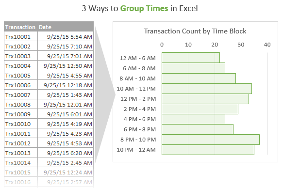
In this article we are going to learn a few different ways to summarize data based on time groups (increments of hours or minutes). This is great if you want to analyze trends throughout the hours of a day to see what time you are busiest, and what time you can take a nap… 🙂 We will also see how to create customized and uneven time blocks.
Download
Download the file to follow along.
The Data Contains a Column with the Date & Time
In this scenario we have a table of sales data that contains one row for each transaction. The second column contains the date and time the transaction occurred.
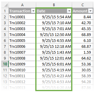
The boss wants to see a report that shows how many transactions took place during each hour of the day. He also wants a report that has groups for every two hours, and another report that combines the overnight hours into one group.
There might be a lot of columns in your data set, but we are really just going to focus on the column that contains the date-time values for this exercise.
Solution #1 – Group Time with a Pivot Table
The quickest and easiest solution would be to use the Group feature in a Pivot Table. This solution is also the most limiting because you will only be able to group the times in 1 hour increments.
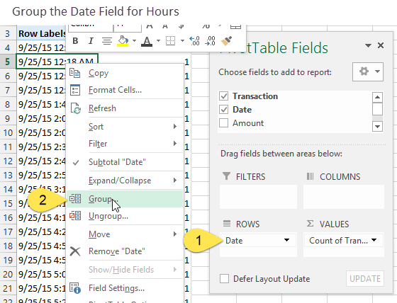
- The first step is to create a pivot table and add the Date field to the Rows area.
- Right-click any cell in the Rows area and choose Group… (Note: if the Group option is disabled then your date field contains text or blanks. All cells in the data column of the data set must contain date values.)
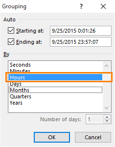
- Choose Hours only from the Grouping menu.
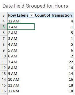
- You should now see a list of one hour increments in the Rows area of the pivot table. The values in the Values area of the pivot table will be summed up to include all transaction that occurred within each hour. The image below shows that there were 4 transaction between 12:00 AM and 12:59 AM.
Please checkout my video series on pivot tables and dashboards for more details on this technique. I explain how to group dates in the 3rd video of that series.
This is a quick solution, but we are only able to group the times in one hour increments. We will have to use a different solution to group the transactions in time blocks of 2 hours or more.
Solution #2 – The FLOOR Function
If the boss wants to see the times grouped in increments other than 1 hour, then we can use the FLOOR function to round the times.
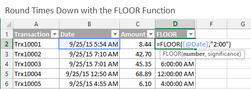
The FLOOR function has two arguments:
=FLOOR(number, significance)
The number is the value to be rounded. In this case it is our date value.
The significance is the multiple to round the number down to. We are also able to specify a time value here.
In this case I specified “2:00” to round the time value down to the nearest 2 hour increment. The nice part is that FLOOR starts at midnight and rounds down in whatever increment you specify. So 12:25 PM and 1:25 PM will both always round to 12:00 PM.
You can also specify smaller increments to group the times by every half hour “0:30” or every five minutes “0:05”.
What If You Have More Than One Day?
If your data set contains sales for more than one day, then you will want to use the TRUNC function to split the time and date. The TRUNC function truncates a number to an integer.

In Excel dates are stored as whole numbers. Dates with times are stored as numbers with decimals. So subtracting the date from the truncated date will return only the decimal number, which is the time.
If you format the date: 9/25/15 5:54 AM as a number you will see: 42272.2460
The 42272 is the date, and the .2460 is the time as a fraction of a day (5 hours 54 minutes).
The number 42,272 represents the number of days that have elapsed since Jan 1, 1900. This is the start of the calendar in Excel.
The [@Date]-TRUNC([@Date] formula returns the .2460, which is the time.
*You will notice that I am using Excel Tables in the image above, but you can use regular cell references as well.
Summarize It With A Pivot Table
This rounding with the FLOOR function has basically assigned a group name to each row of the source data.
You can now add the column that uses the FLOOR function in the Rows area of the Pivot Table, instead of the Grouped Date field.
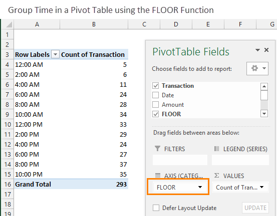
This gives us a summary of the transaction count by two hour blocks. If your data set spans multiple days then this is really going to show you what times of the day you do the most volume. You could analyze it further to see the days of the week, weeks in the month, etc.
Solution #3 – The VLOOKUP Function
What if we don't want the same amount of time for each group? In the image at the beginning of the article I show a report that has a time block from 12 AM – 6 AM (6 hours), then 2 hour intervals for the rest of the day.
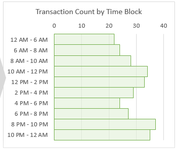
The boss might want to see it like this because there isn't much business overnight, and it takes up a lot of space on the report or chart.
Use VLOOKUP To Return The Closest Match – Grouping Technique
For this solution we can use VLOOKUP to lookup the time in a lookup table.

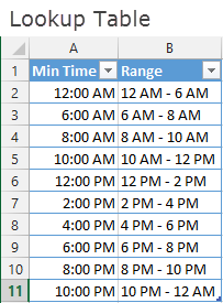
The first column in our lookup table contains the time value to lookup. The second value contains a group name. This is just text that I created with a formula using the TEXT function.
Notice that the last argument in my VLOOKUP formula is TRUE, which means we are using it to return a closest match. Here is an article on returning the closest match with VLOOKUP. It's a great technique to learn for things like calculating commissions or tax rates.
If you are completely new to VLOOKUP checkout this article where I explain VLOOKUP at Starbucks.
Summarize the Uneven Time Groups with a Pivot Table
Adding the column with the VLOOKUP formulas to the Rows Area of the pivot table gives us a summary of transaction based on the uneven time groups.
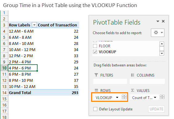
One drawback to this method is that you will have to manually sort the group names in the Rows Area of the pivot table. These group names are text, not numbers, so Excel will not be able to sort them as times.
Conclusion
There are a lot of ways to group times in Excel. The quickest and easiest method is probably to use the Group feature in a Pivot Table (solution #1). If you want to group the times in increments of multiple hours or fractions of an hour, then the FLOOR and VLOOKUP functions can help group the times.
Please leave a comment below with any questions. Thanks!




I am having issues in my files even though I followed the steps. I can share the worksheet.