How to Calculate Commissions in Excel with VLOOKUP, XLOOKUP, or IF

Bottom line: Learn how to calculate commissions in Excel for a basic tiered plan and rate table using the IF, VLOOKUP, or XLOOKUP functions.

Skill level: Intermediate

Video Tutorial

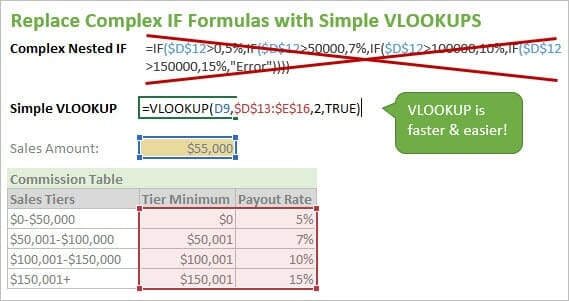
Calculating commissions in Excel can be a very tricky task.  This is especially true if you have tried to use multiple IF statements to calculate commissions for each tier in a rate table.

This article will explain how to use the VLOOKUP function to make this process much easier.  The secret is setting the last argument in the vlookup to TRUE, to find the closest match.

Please checkout my article on How to Use VLOOKUP to Find the Closest Match for a detailed explanation on setting the last argument to TRUE.

Update: The post has been updated to include instructions for calculating commissions with the new XLOOKUP function. Here is an article & video on XLOOKUP.

Download File

Download the file to follow along.

Calculating Commissions with VLOOKUP

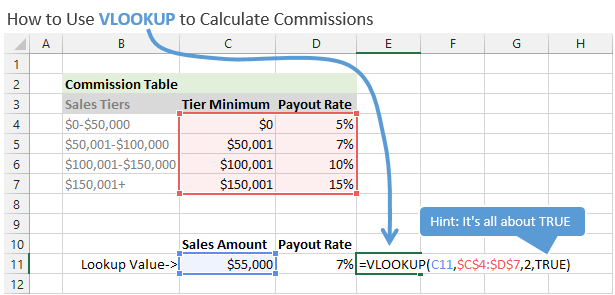
With a simple commission plan you typically have a rate table that lists the payout rate at each level of sales.  As the sales rep makes more sales, his/her payout rate will typically increase.

The payout rate could be a flat dollar amount, percentage of revenue, percentage of quota, etc.  The job of the VLOOKUP is to find the rep's sales amount in the rate table, and return the corresponding payout rate.

For this example our commissions plan looks like the following:

• Rep sells $0-$50,000, they earn 5%
• Rep sells $51,000-$100,000, they earn 7%
• Rep sells $100,001-$150,000, they earn 10%
• Rep sells over $150,001, they earn 15%

The rep will make a certain amount of sales during the month.  He/she will earn a certain payout rate depending on the level of sales achieved.

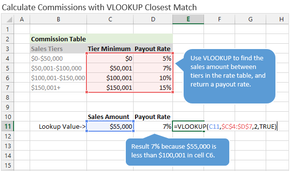
We can use a VLOOKUP formula to calculate the payout rate for a given sales amount (lookup value).  For this to work we need to set the last argument in the vlookup [range_lookup] to TRUE.

With the last argument set to TRUE, vlookup will find the closest match to the lookup value that is less than or equal to the lookup amount.  This basically allows us to find a value between ranges of two numbers (tiers).

This is why the last argument in VLOOKUP is named range_lookup. When this argument is TRUE, VLOOKUP is looking between ranges of values in the tier minimum column to find an exact match or the value less than the lookup value.

How to Setup the Rate Table

When putting this rate table in Excel, you only need to list the tier minimum for the lookup range.  Again the VLOOKUP will search for a “closest match” that is less than or equal to the lookup value.  If it finds a value that is greater than the lookup value, then it will return the previous row.

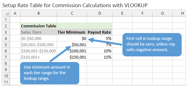
In this example for a commissions rate table, the first row in the lookup range needs to be zero.  This is because the sales rep could potentially have sales of $0 and the lookup value would be zero.  If the lookup value (sales amount) were a negative number, then the vlookup would return an error.

It is important to know this and setup your rate table for all possible lookup values.

If the sales amount is greater than the last row in the lookup range, then the vlookup will return the last row.  For example, if the rep made sales of $175,000 then vlookup would return 15%.

Calculate Commissions to Return a Dollar Value

The payout can also be returned as a dollar value, instead of a percentage.  With this setup the payout will be a flat rate.

This means that the payout will be the same, regardless of what the sales amount is within the tier.  In the example below, if the payout will be $1,000 if the sales amount is $55,000 or $95,000.

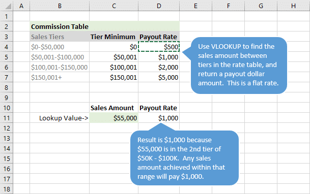
The payout is NOT on a sliding scale.  It is a flat rate for each tier.

If you are looking for a sliding scale calculation, see my article on calculating commission with a tiered rate structure using SUMPRODUCT.

Commission Calculations with XLOOKUP

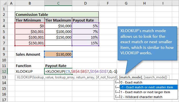
We can also use the new XLOOKUP function for this calculation. It works very similar to VLOOKUP when finding the closest match.

Advantages with XLOOKUP

There are two main differences and advantages with XLOOKUP:

1. With XLOOKUP we specify the lookup array and return array as separate ranges. This is B4:B7 and D4:D7 in the image above. This is an advantage over VLOOKUP because we can insert or delete rows between columns B and D, and the formula will still work.
   
   When we add/delete columns within the table array of VLOOKUP, we have to manually change the column index number or use a formula to dynamically calculate it.
   
2. XLOOKUP does NOT require the data to be sorted when using Exact match or next smaller/larger item for match mode. XLOOKUP will actually look for the next smaller/larger item and return the result from that row/column.
   
   VLOOKUP requires the data to be sorted when the last argument is TRUE. Typically you will want to sort your data for these types of tables anyways, but it's good to know that you can just put new rate tiers at the bottom of the table and XLOOKUP will work.

Drawback of XLOOKUP

The main disadvantage with XLOOKUP is compatibility. Both you and all of the users of your file must be on a version of Microsoft/Office 365 that has XLOOKUP. It's is NOT backward compatible or available on older versions of Excel.

Therefore, VLOOKUP works great in this scenario and is much easier to write than a nested IF formula.

Avoid Nested IF Formulas

A common approach to calculating commissions is using IF statements.  With a rate table like this you would have to write multiple IF statements.  You basically have to write one IF statement for each tier (row) in the table.

You then have to join all the IF statements into one long and ugly formula.  These are called nested IF statements.

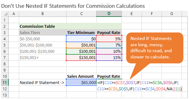
I always try to avoid nested IFs when possible because they are difficult to read and understand, and they can be slower for Excel to calculate.  If you have thousands of nested IF formulas in your workbook, your calculation time could slow down.

The IF formula is much more difficult to maintain. It requires modification when rows are added/deleted from the table. VLOOKUP and XLOOKUP do NOT require this type of maintenance.

If you do use IF, make sure to make each cell reference to the rate table an absolute reference (F4 on the keyboard). Otherwise you will get incorrect results when copying the formula down.

Using VLOOKUP is much easier and cleaner than using nested IF formulas.  As you can see with this example, the vlookup allows you to use one formula to calculate the commission payout rate for any given sales amount.

Additional Resources

• How to Use VLOOKUP to Find the Closest Match – Last Argument Equals TRUE
• How to Calculate Cumulative Tiered Commissions with SUMPRODUCT
• VLOOKUP Explained in Simple Terms at Starbucks
• VLOOKUP & MATCH – A Dynamic Duo
• The New XLOOKUP Function for Excel + Video Tutorial
• IF Function Explained: How to Write an IF Statement Formula in Excel

How Do You Use VLOOKUP with Closest Match?

The VLOOKUP with closest match technique can also be used for tax bracket calculations, price matching, etc.  What do you use this technique to calculate?

Please leave a comment below with any questions or suggestions.  Thanks!