Bottom Line: Learn how to use the IF Function to write formulas that return results based on a condition or logical test. This post includes training on logical tests, comparison operators, nested IF formulas, multiple conditions with AND and OR functions, and common causes of formula errors.
Skill Level: Beginner
Watch the Tutorial
Download the Excel File
You can access the file that I use in the video by clicking below.
Mastering the IF Function
The IF Function is an important function to know. It can help with comparing data, performing lookups to group data, and making reports interactive. If you're not familiar with IF or could use a refresher, this post will help.
Here is the IF function's signature:
=IF(logical_test, [value_if_true], [value_if_false])
The IF Function has 3 arguments:
- Logical test. This is where we can compare data or see if a condition is met.
- Value if true. Defining this argument tells Excel to return a certain value if the condition in the logical test is met.
- Value if false. If the condition is not met, this argument defines what the returned value will be.
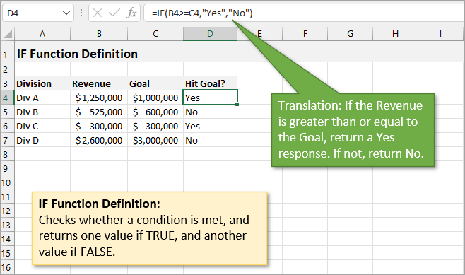
Here's an example. I'm comparing Revenue amounts with Goal amounts. If the Revenue is greater than or equal to the goal, I want column D to say Yes, and if not, to say No.
Let's talk about the most important part of the IF function: the logical test.
Logical Tests
The logical test portion of the formula always uses a comparison operator to compare values and determine if the statement is true or false. Here is a list of comparison operators that can be used.
| Operator | Description |
|---|---|
| = | Equal To |
| <> | Not Equal To |
| > | Greater Than |
| < | Less Than |
| >= | Greater Than or Equal To |
| <= | Less Than or Equal To |
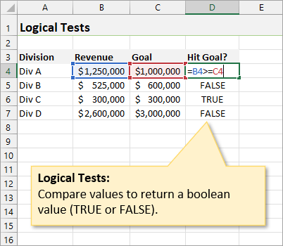
Logical tests return TRUE or FALSE values. This is important because the logical test argument within IF needs a TRUE or FALSE (boolean) value returned to it. It is also important because you might not even need an IF function if the TRUE/FALSE values can be used to get the answer you are looking for.
It's also important to note that the case doesn't matter when comparing text. The following formula will return TRUE.
=”Excel Campus” = “excel campus”
Returning Other Values
While “TRUE” and “FALSE” would probably be sufficient for my example, I prefer them to say “Yes” and “No” in answer to the question in by column header: “Hit goal?”.
The advantage of using an IF function is that you can return any values you like by specifying the words that you want to appear. Just make sure to wrap them in quotation marks when writing your IF formula, unless they are numbers. If you do not specify these second and third arguments when writing the IF formula, it will simply return TRUE and FALSE.
The value_if_true and value_if_false arguments can contain just about anything:
- A number
- Text wrapped in double quotes – “hello”
- A reference to another cell – A2
- A formula with another IF function.
- A formula with any other combination of functions.
It's also important to note that both the value_if_true and value_if_false arguments are optional. This is denoted by the square brackets around them in the function signature.
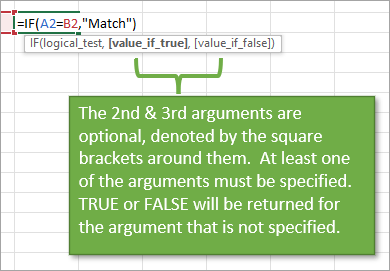
You must specify at least one of the arguments. If you leave one of the arguments blank and the logical test results in that condition, then a TRUE or FALSE value will be returned to the cell.
For example, the following formula will return a FALSE if A2 does NOT equal B2 because the value_if_false argument is not specified.
=IF(A2=B2, "Match")
Grouping Data
One common use for the IF Function is to categorize data. Let me show you an example.
On this worksheet, I want to categorize transactions as either Large or Small depending on the amount I've entered in cell D4. A transaction less than $60,000 will be labeled as small. Transactions greater than or equal to $60,000 will be large.
When writing the formula, I could specify the amounts and the labels by typing them out, but I prefer to use cell references so that they can quickly and easily be updated without rewriting the formulas.
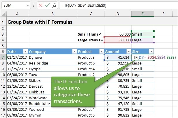
The dollar symbols ($) in the formula make the references absolute so that they don't change when the formula is copied down to the cells below it. When the cell reference within the formula is selected, you can hit F4 on your keyboard (for Fn + F4 for most laptop keyboards) to insert a dollar symbol before the row number and column letter. (Pressing it repeatedly will toggle it to one or the other and back again to none or both.)
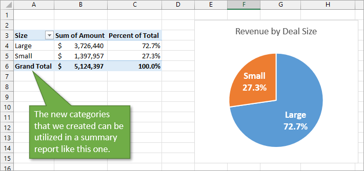
Categorizing these transactions is helpful for analyzing the data. You can filter out just the large or small items, or you can use these labels in a summary report, pivot table, or chart. Below is an example.
Multiple Logical Tests
If we want to use more than one logical test, we can use the AND and OR Functions.
The AND Function
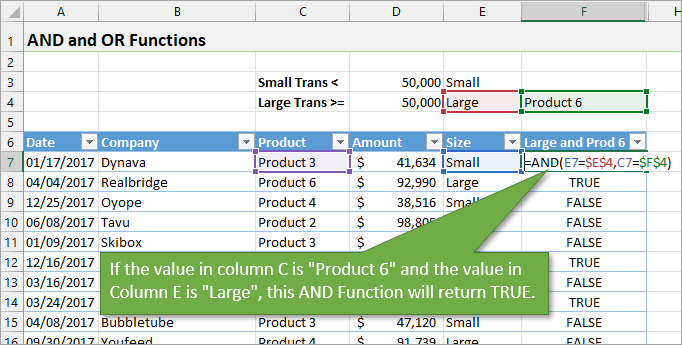
The AND Function checks whether all arguments are true and returns TRUE if they are.
In the example below, our formula is looking for transactions that are both “Large” and “Product 6.”
The OR Function
Perhaps you want show a positive result if only ONE of the logical tests in your formula is true, not BOTH. If that is the case, you can use the OR Function.
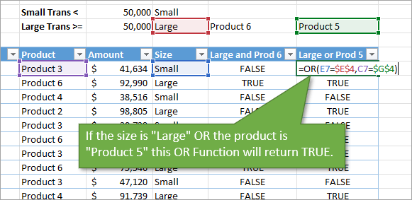
The OR Function checks whether any of the arguments are true, and returns TRUE or FALSE. It returns FALSE only if all arguments are false.
Using the same sheet as above, the formula in our example below is looking for entries where the size is “Large” OR if the product name is “Product 5.”
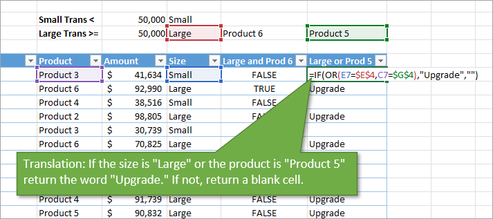
If we want to return text or a number instead of TRUE or FALSE, then we can wrap the AND or OR Functions in the IF Function. For example, using the OR Function above as our logical test in an IF Formula, we can type the word Upgrade (in parentheses) as our Value If True argument. That means, when the conditions we've specified are true, the cell will say Upgrade. To return a blank cell when the conditions aren't met, we just have two quotation marks with nothing between them for our Value If False argument.
Nested IF Formulas
Things can get more complicated when there are more categories added to the mix. Maybe you want to group data based on 3 or more logical tests in your IF formula.
When this happens, we end up nesting another IF Function into our existing function each time we add another category.
For example, let's say we have three account categories called Small, Large, and Key. A Small account is less than $10,000. A Large account is between $10,000 and $70,000. And a Key account is more than $70,000.
When we write our formula to categorize these accounts, we will need to use two IF statements, with one nested within the other.
The logic of the formula goes like this.
- If the amount is greater than or equal to $70,000, return a value of “Key.”
- But if it's NOT, evaluate the next IF Function.
- If the amount is greater than or equal to $10,000, return a value of “Large.”
- But if it's NOT, return a value of “Small.”
With the cell references plugged in for the sizes and amounts, the formula would look like this on our spreadsheet.
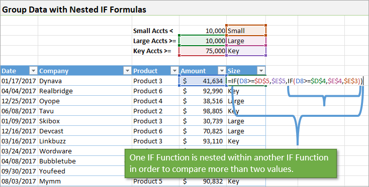
As you can imagine, these nested IF formulas can get longer and uglier with each additional category or criteria that is added. That being the case, there are a couple of alternatives that I would like to mention.
Alternative 1: The IFS Function
This is a relatively new function introduced in Excel 2019. While it still requires a lot of selection and logical tests, it is somewhat easier to read and write the IFS formula compared to nested IF formulas.
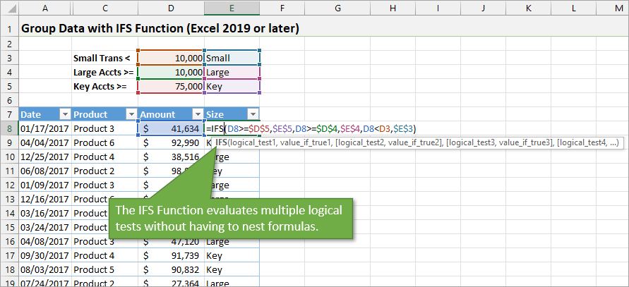
I won't go into detail about writing the IFS Function, but you can play around with it in the Excel file attached at the top of this post.
Alternative 2: Lookup Formulas
You can use VLOOKUP, XLOOKUP, or Index Match to return the same results as the nested IFs. These are a lot simpler to write. For an explanation of how to write a VLOOKUP formula like this, jump over to this tutorial:
How to Use VLOOKUP to Find the Closest Match – Last Argument is TRUE
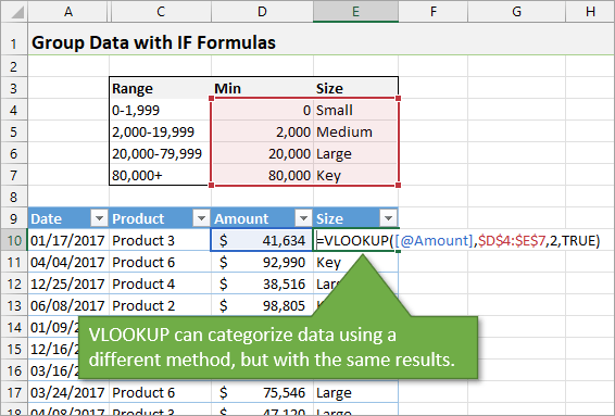
Common Errors with the IF Function
If you come across errors when using the IF Function, it is most likely related to data types. What I mean by that is, Excel can't compare text to a number or a date, or evaluate text that is different. However, the formatting of values doesn't hinder Excel from making comparisons in logical tests. Below you can see how the values in Column A and Column B return a TRUE or FALSE in column C when they are compared.
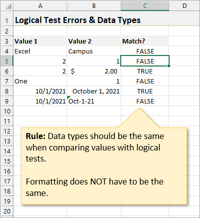
Note that while the entry in B9 looks like it is formatted as a date, it is formatted as text. That is why it is returning FALSE when compared to the date in A9. See the video above for a further explanation on errors with data types.
Related Posts
If you found this information helpful, check out these other tutorials on related content.
- How to Calculate Commissions in Excel with VLOOKUP, XLOOKUP, or IF
- Introduction to Pivot Tables and Dashboards
- Excel Tables Tutorial Video – Beginners Guide for Windows & Mac
Conclusion
Ready for a challenge? Test what you've learned and get more practice by taking our free IF Formula Challenge! You can access it here:
The challenge includes videos that explain the challenge and walk through the solution. See if you can earn all six gold stars in the challenge file.
I hope this explanation has been helpful and that you start putting the IF Function to work in your spreadsheets soon if you're not already using it. Leave a comment below if you have questions or feedback!


Thanks Jon! It’s nice and clear, A special Thanks for the Challenge sheet!!
What’s the real benefit I gain from IFS vs Nested IF?
Thanks. I learned a lot.
Hi Jon
Very detailed presentation of the progressive donut chart, loved it.
Question: I have a group of supervisors providing monthly trainings and I would like to add those trainings or perecentage per month in the same chart. Would that be possible?
I am trying to get cell 1 to equal the dollar amount in cell 2 if the cell 3 has a value over $0.00
Hi Jon,
Maybe you can help me or anyone more inspired than me at this point. 🙂
In Excel I have to apply a sort of statistical calculation to a row considering the expression:
T=(t1^3-t1)+(t2^3-t2)+……+(t_11^3-t11)
where t = the number of appearances in the range for a certain value.
For example, in row 1 there are the numbers: 2, 3, 3, 7, 1, 5, 5, 5, 4, 4, 6.
Manually, first I would take each number in the range and look if it’s a duplicate.
Number 2 is a unique value, appears only 1 time in the range, so the calculation is: 1^3-1=0.
Number 3 is a duplicate, appears 2 times in the range, the calculation is: 2^3-2=6.
Number 7, number 1 – same as number 2.
Number 5 is a duplicate, appears 3 times: 3^3-3=24; etc….
Once done with all the numbers in the range, then sum up all the values calculated before.
Any idea how this can be done in Excel, avoiding all this manual labor?
Thanks in advance for your replies.
All the best!
Hi. Can i check if i want to get a payout of 3 different amount using 8 types of values, what should the formula be?
Criteria :
Total Chats – 1000
Satisfaction – 80%
Response Time – 30 sec
Total Email – 1000
Satisfaction – 80%
Response Time – 30 sec
Total Call – 1000
Total Review – 80
Payout :
$1000
$500
$0
To get a payout of $1000, you must have 1000 chats or above.. satisfaction more than 80%.. response time less than 30 sec.. total email 1000 or more.. satisfaction more than 80%.. response time less than 30 sec.. Total call of 1000 or more.. Review with 80 or more..
But if you only achieve a total of 1000 chats, 1000 emails, 1000 calls and 80 reviews, but the satisfaction and response did not meet, you can only get a payout of $500..
Lastly if all 8 criteria did not meet, you will get $0
Excellent explanation!!! Thanks a lot.
I can not download the file; could you please tell me how to do it?