How to Remove Errors in Your Pivot Tables + Video

Bottom line: Learn how to remove or replace the error values in your pivot tables.  You will also learn how the Pivot Layouts feature of the PivotPal Add-in can save a lot of time with pivot table settings.

Skill level: Beginner

Handling Errors in the Pivot Table Values Area

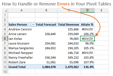
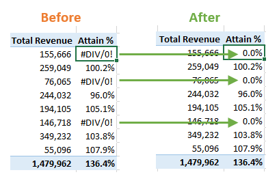
The most common type of error I see in the values of a pivot table is Divide by Zero (#Div/0).  This error is typically caused by a calculated field or calculation on a field (show values as option).

Displaying the error can make our pivot tables look ugly.  Fortunately, there is a way to remove or replace the error.

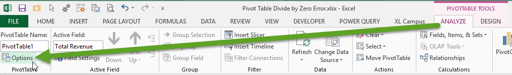
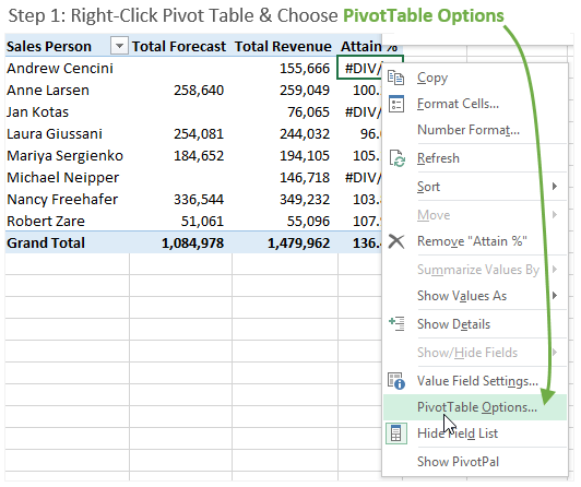
Step 1: Open the Pivot Table Options Menu

The PivotTable Options menu can be found on the left side of the Analyze/Options tab in the ribbon when any cell is selected in the pivot table.

You can also Right-Click on the pivot table and choose PivotTable Options.

Step 2: For Error Values Show Checkbox

The “For error values show” option on the Layout & Format tab of the PivotTable Options will allow you to handle the errors.

Once the box is checked, the value in the text box to the right will be displayed in the pivot table.  You can put a number or text in this box.  The error values in the pivot table will be replaced with whatever you put in the text box.

You can also leave the box blank to display a blank cell in the pivot table.

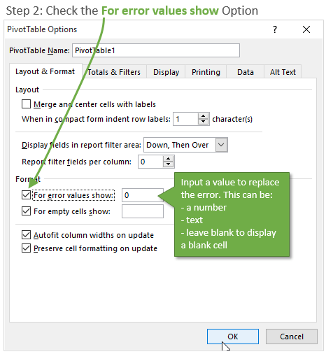
Press OK after you have made your changes and the pivot table will display the changes.

Unchecking the option will display the errors again.

Here is a before and after of what the pivot table looks like when displaying zero for errors.  As you can see, the number formatting is also displayed for the zero values.  The field is formatted as a percent, and the zeros are formatted as a percent as well.

Save Time with PivotPal & My Pivot Layouts

By default, the “For error values show option” is unchecked.  This can be good because it lets you know that there are errors in your calculations.  But it can also be annoying to have to go change this setting, or any of the other 30+ pivot table options, every time you create a pivot table.

In the video above I demonstrate how the My Pivot Layouts feature of PivotPal will save you a lot of time when modifying the settings of your pivot tables.  You can create custom profiles that save all of your pivot table settings, and then quickly apply all the settings to your pivot tables at one time.

This feature will save you a ton of time!

Try PivotPal Today

This week you can save 20% on PivotPal when you use the code layout20 at checkout.  The discount expires on Sunday August 23rd at midnight PST.

Click Here to Get PivotPal Today

Please leave a comment below with any questions.  Thanks!