How to Compare Two Sheets in Excel: Bank Reconciliations Made Easy

Bottom Line: Simplify your bank reconciliations by using Excel’s pivot tables to compare data sets, identify discrepancies, and create clear, actionable reports.

Skill Level: Intermediate

Watch the Tutorial

Download the Example File

You can follow along using the same Excel file that I used in the video.

Make Reconciliation Easier

A bank reconciliation is the process of finding differences between a bank statement and the accounting system. Of course, the goal is for everything to match and tie out perfectly. But in the real world, that isn't always the case.

Reconciliation can feel like finding a needle in a haystack, especially when you’re working with hundreds (or thousands!) of transactions.

Excel’s pivot tables make it easier to compare two datasets, like bank statements and accounting records, to spot and resolve discrepancies. In this post, we’ll walk you through how to set up and analyze your data for a smoother reconciliation process.

Step 1: Combine Your Data Sets

The first step is to bring all your data into one table. Here’s how:

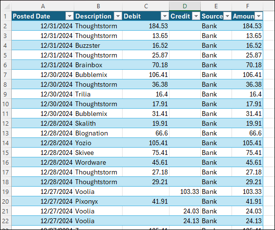
1. Prepare your bank statement data:
   • Save your bank statement as an Excel file.
   • Insert a table by selecting the data and pressing Ctrl + T.
   • Add a column labeled Source and populate it with “Bank” to identify the rows as originating from the bank statement.
   • Add a column for Amount in which you add the debit and credit columns.

So far, your worksheet should look something like this:

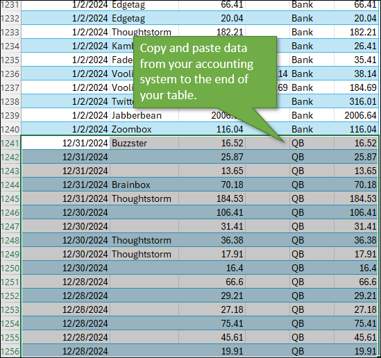
2. Prepare your accounting system data:
   • Export your data from your accounting software (e.g., QuickBooks).
   • Copy and paste the data into the same table below the bank statement data.
   • Populate the Source column with a label like “Accounting” or “QuickBooks.”

---

Step 2: Create a Pivot Table

Once your data is in one table, you can create a pivot table. If you're not familiar with pivot tables, here's a good place to start. To create the pivot table:

1. Select any cell in the table and go to Insert > Pivot Table.
2. Choose to place the pivot table on a new worksheet.

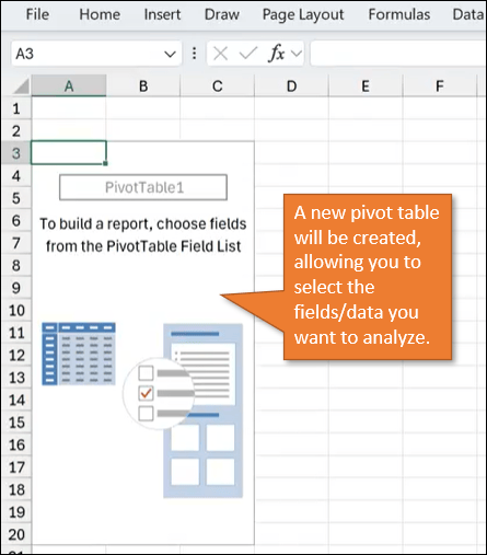
Now you’re ready to build out your table and analyze your data.

---

Step 3: Analyze the Data with a Pivot Table

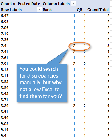
Identify Total Transactions

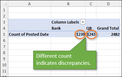
• In the Pivot Table task pane, drag the Source field into the Columns area.
• Then drag the Posted Date field into the Values area.
  This will give you a count of transactions for each source. Any differences in totals indicate discrepancies.

List All Transactions

• Drag the Amount field into the Rows area.
  This creates a list of all transaction amounts from both sources, showing where discrepancies occur.

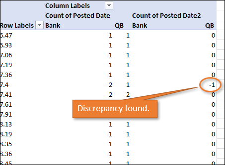
Highlight Discrepancies

• Add the Posted Date field to the Values area again and set it to Show Values As > Difference From, using the right-click menu.
• Then, use the Source field as the base field to calculate differences between sources.

This will show where counts differ between the datasets, indicating transactions that need investigation.

---

Step 4: Drill Down for Details

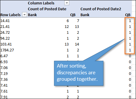
Sort and Filter Discrepancies

• Sort the pivot table to group discrepancies (non-zero differences) together.
• Positive numbers will be at the top of your list and negative numbers will be at the bottom. Both are discrepancies to be fixed and the only difference between positive and negative is which data source had more entries.

See the video above for detailed instructions on how to do this sort.

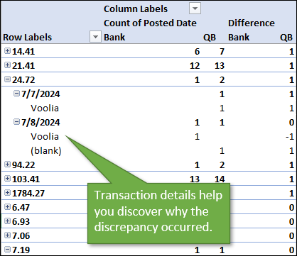
Expand for More Context

• Drag the Posted Date filed into the Rows area.
• Then, drag the Description field into the Rows area below the Posted Date field.
  This reveals transaction dates and vendor names or other relevant details, helping you locate the stray transactions in your bank or accounting system.

---

Step 5: Resolve and Refine

Once you’ve identified the discrepancies, investigate further:

• Transactions missing: Check for items not imported into your accounting system.
• Duplicates: Identify duplicate transactions that may need removal.
• Date mismatches: Look for transactions posted on different dates in the two systems.

---

Bonus Tips

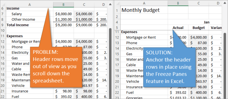
Freeze Headers for Easier Navigation

Freeze panes on the header row of your pivot table to keep it visible while scrolling.

Here's a post that shows you how to freeze panes.

Automate Frequent Reconciliations

If this process is a recurring task, consider automating the data import and combination steps. I'll teach you how to do that in my next tutorial.

---

Conclusion

With just a bit of setup, Excel’s pivot tables make reconciling accounts faster and more accurate. By combining data into one table and leveraging the pivot table’s powerful analysis capability, you can spot discrepancies, drill down for details, and create clear reports—all without complex formulas.

Do you find this reconciliation process useful? Leave a comment below and let us know!