New Excel Slicer for PIVOTBY

Bottom Line: Learn to create a new type of slicer or filter that you can use to make interactive reports and dashboards in Excel.

Skill Level: Intermediate

Watch the Video Tutorial

Download the Excel Files

You can follow along using the following Excel files.

In today's tutorial, we'll explore a new approach to slicers for creating interactive reports and dashboards in Excel. Microsoft recently introduced GROUPBY and PIVOTBY functions, alternatives to pivot tables for data analysis and summary reports. However, these new functions lack slicers for interactivity.

To address this, we'll build a Dynamic Grid Slicer as a workaround.

Let's dive into the details.

Understanding the Setup

To set the stage, we have a summary report generated by the new PIVOTBY function. This function is pulling from source data containing order details. The report shows the number of units sold by color and with a year-over-year comparison.

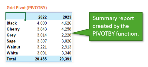
From this table, I've created a simple bar chart to display the data visually.

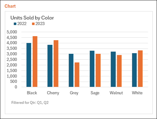
With a normal pivot table, we can easily add slicers, which allow us to filter data down, but that's not the case with a PIVOTBY table. So we're going to replicate the interactivity of regular pivot tables and slicers using a combination of formulas and checkboxes.

Dynamic Grid Slicer Features

Our Dynamic Grid Slicer mimics the functionality of regular slicers. It includes a dropdown button for selecting columns, checkboxes for applying filters, and automatic recalculation when source data changes.

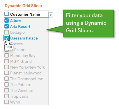
The term “dynamic” in the slicer's name comes from its ability to adapt to changes in the source data. Unlike traditional slicers, the Dynamic Grid Slicer offers automatic refresh and recalculation, ensuring real-time updates without manual intervention.

Creating the Dynamic Grid Slicer

Let's look into the process of creating the Dynamic Grid Slicer. While using a regular pivot table and slicer is easier, this tutorial accomodates those who prefer a formula-based approach. Even if you don't plan to use Dynamic Grid Slicers, you'll learn valuable techniques for dynamic array formulas.

I'll address the challenges with GROUPBY and PIVOTBY in an upcoming video, so be on the lookout for that in the future.

Setup and Formulas

Let's explore the setup for the Dynamic Grid Slicer. We need a list of unique values that will be used to create the filter list. The UNIQUE function, combined with the INDIRECT function for dynamic referencing, helps create a list of unique values for user filters.

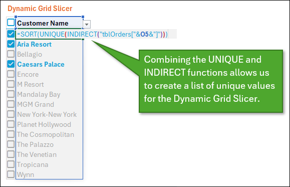
Additionally, a hidden column with the FILTER function generates a list of values where the checkbox has been checked. This list will be used for the Filter argument in PIVOTBY. The overflowing spill range ensures dynamic updates as the list changes.

Applying Filters in PIVOTBY

To apply filters in PIVOTBY, we use the filter_array argument. A complex formula using ISNUMBER and XMATCH facilitates the filtering process, ensuring that the results dynamically adjust to the selected values in the Dynamic Grid Slicer.

For a more detailed explanation of each part of this formula, watch the video at the top of this tutorial.

The checkboxes are added using the Checkboxes in Cells feature, found on the Insert tab of the Ribbon.

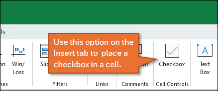
Watch this tutorial for more information about how to add checkboxes: New Checkboxes in Excel.

You can use conditional formatting to make invisible the entries that aren't being displayed for each filter list. You can see the various rules that I use listed under Conditional Formatting in the Excel file I've provided above.

Bonus Features

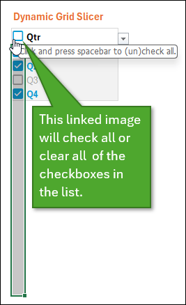
In an attempt to recreate the Clear-All button on a regular slicer, I've added a button at the top of the Dynamic Grid Slicer that allows us to reset all filters.

This button is actually just an image of a checkbox, which is linked to a named range that includes all of the checkboxes. So by clicking the spacebar, you can check or uncheck all of the checkboxes in the list.

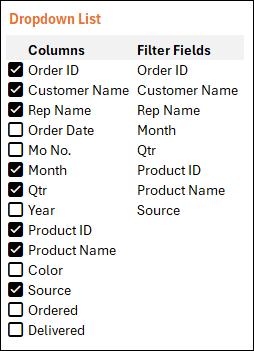
Moreover, we can limit dropdown columns using another Dynamic Grid Slicer. Using the slicer below, I simply check or uncheck the column names that I want to be available for filtering in the dropdown list of my first slicer.

Feel free to experiment with multiple grid slicers on a sheet. Again, the file used in this tutorial is available for free download above.

Note

Both PIVOTBY and the new checkboxes are on the Beta channel for Microsoft 365 at this time. Hopefully, we will see wider availability in a future release soon.

Conclusion

Thanks for reading this tutorial on creating interactive and dynamic reports with the new PIVOTBY function. Please share your thoughts and questions in the comments below, and stay tuned for our upcoming video comparing PIVOTBY and GROUPBY with regular pivot tables.

Have a great day!