Budget Makeover – Ep. 4 – Using Freeze Panes in Excel

Bottom Line: Learn how to lock rows and columns when scrolling with the freeze panes feature.

Skill Level: Beginner

Watch the Tutorial

Download the Excel Files

You can access both the BEFORE and AFTER Excel files to follow along:

Making Budgets Better

Welcome to the fourth episode in our Budget Makeover video series. Earlier in the series, we learned how to:

1. Lock Cells and Protect Worksheets
2. Remove Duplicate Entries to Make a Unique List
3. Create Dropdown (Data Validation) Lists

Today, we'll take a look at freezing panes so that certain rows and columns stay static when scrolling through a worksheet.

How to Freeze Panes

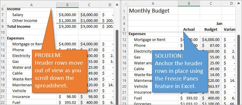
Some budgets can be pretty lengthy, and it's frustrating when you can't readily see the column headers as you are trying to look at the numbers lower down on the page. It's the same for row headers as you navigate further and further to the right.

Fortunately, Excel has an easy way to lock rows and columns in place so that they are always visible, no matter where you scroll. It's called freezing panes.

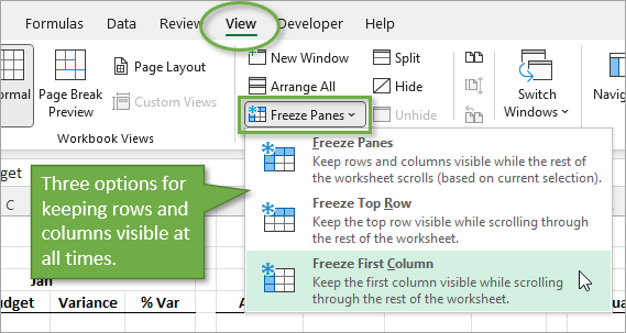
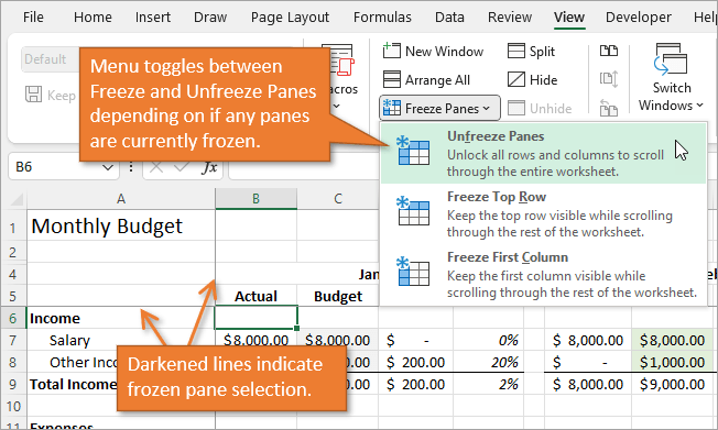
To freeze panes, simply go to the View tab on the Ribbon and select Freeze Panes. You will notice there are three options:

1. Freeze panes (to keep rows and columns visible)
2. Freeze the top row
3. Freeze the first column

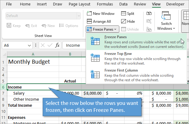
Options 2 and 3 only freeze the FIRST row or column. There are many times, however, when you want several of the first rows or columns to remain visible. For example, I want the first five rows in our spreadsheet to be frozen in place. To do that, I just select the row below my desired selection (Row 6) and then choose Freeze Panes.

The same procedure applies to freezing multiple COLUMNS, except you start by selecting the column to the RIGHT of the columns you want frozen.

You may want header rows AND columns to be frozen simultaneously. If so, start by selecting the cell to the right of your desired columns and below your desired rows. Then click on Freeze Panes.

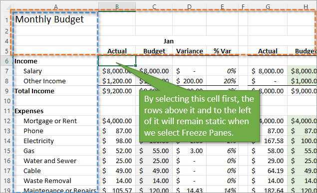
The gridlines on the edge of your frozen panes will be slightly thicker/darker than normal as a visual indication of which rows/columns are frozen.

Unfreeze Panes

If you want to change which panes you want frozen, you will have to unfreeze your existing selection first. Whenever you have frozen panes, the option to Unfreeze Panes will take the place of Freeze Panes in the dropdown menu.

Keyboard Shortcut

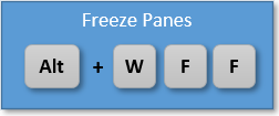
The keyboard shortcut to freeze panes on Windows is Alt + W, F, F.

Conclusion

As you can imagine, this simple process is not only valuable for reviewing budgets but for navigating spreadsheets in general. I hope it proves helpful to you. If you have questions or comments, write them below and we will respond.

I've got a related post that might interest you. It's about how to take care of situations when gridlines and freeze panes don't transfer to a new window. Gridlines & Freeze Panes Settings Lost in New Window – How to Fix It

Our next step in the budget makeover process is to learn how to write a SUMIFS formula to create summary reports, sum by category, and time period.

Episode 1: Budget Makeover – Ep. 1 – How to Lock Cells for Editing in Excel

Episode 2: Budget Makeover – Ep. 2 – How to Remove Duplicates in Excel

Episode 3: Budget Makeover – Ep. 3 – Creating Dropdown Lists