Attendance Report Dashboard for All Versions of Excel

Bottom Line: Learn to create an interactive dashboard for employee attendance using Excel 2010 or beyond.

Skill Level: Intermediate

Download the Excel File

The Excel file I used in this post can be downloaded here:

Update: I opened the file in Excel 2010 and did not like how the transparent shapes look when pasted as a picture.  The shape looks like a gray box instead of just adding white transparency.

So I created another version that uses two different icons on the Shapes sheet.  I used the Color drop-down on the Picture Format tab to change the color saturation of the “bad” shape to give it a grayed-out look. 

Here is the file that contains that solution.

Office 365 Alternative

As part of an Excel Hash competition, I submitted a winning entry featuring an attendance dashboard. This dashboard report was a parody of something Dwight Schrute would use in the TV show The Office. You can see the entry explained here: Excel Hash: Attendance Report with Storm Clouds & Fireworks.

That solution uses new features that only available in the latest versions of Excel:

1. XOR – Excel 2013
2. Icons – Excel 2016
3. Dynamic Arrays Functions (FILTER, UNIQUE, SORTBY) – Office 365
4. XLOOKUP – Office 365

However, a lot of readers aren't running that newest version of Excel, so I've created this post as an alternative that can be used with older versions of Excel.

I've created six video tutorials that walk you through the creation of that dashboard. Even if you don't have Office 365, I recommend viewing them as they will help to give you context and detail. Then come back here and see how I adapt the process. We can use other formulas and workarounds to create the same report with Excel 2010 or beyond. It should work in 2007 as well but I have not tested.

The first video in that series can be found here: How to Use the XOR Function

Setting Up the Source Data

In the original series of posts, I use the XOR function to determine if the attendance data entries were “In” or “Out” entries. We could figure that out depending on whether there was an even or odd amount of entries.

We can accomplish the same thing using the ISEVEN and COUNTIF functions.

The first thing we need to do is sort the data from newest to oldest instead of the other way around. With XLOOKUP, we had the ability to search in reverse order. But since we are using an older version of Excel, we will use VLOOKUP instead. VLOOKUP can't search in reverse order. Here is a post about VLOOKUP if you want to know more about it: VLOOKUP Explained.

Using VLOOKUP, we can find the previous date in order to calculate the duration.

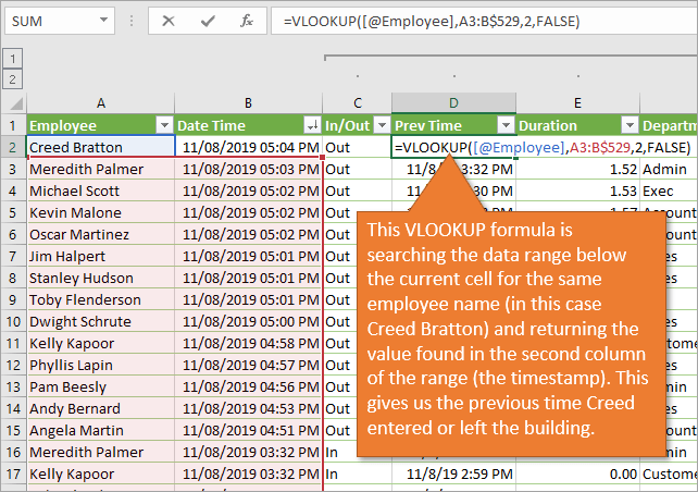
To calculate the duration, we subtract the prior “In” timestamp from each “Out” timestamp and multiply by 24 to get the number of hours the employee was at work.

COUNTIF for Distinct Count

We also need to calculate the average duration for all employees in the selected department. We are going to use a pivot table for this, which is explained below.

The pivot table needs to calculate the distinct count of number of employees in the selected department, so the average can be calculated.

Average Duration = Total Hours / Count of Employees

Excel 2010 and earlier does not have the ability to calculate distinct count directly in the pivot table. So we can use a formula in the source data instead.

=1/COUNTIF([Employee],[@Employee])

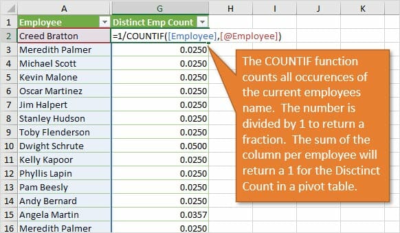
This returns a decimal number for each row. When the row is summed it will return a 1 to the pivot table for each employee in the rows area, based on the filter criteria for the selected department.

I've got another blog post that takes a closer look at the COUNTIF function: How to Use the COUNTIF Function.

Summarizing with Pivot Tables

To create the same interaction on the dashboard that the original worksheet features, we can use pivot tables and a slicer instead of Dynamic Array Functions. If you're not familiar with pivot tables, you'll want to be. They are really useful. You can learn more about how to use pivot tables in this post: Introduction to Pivot Tables and Dashboards.

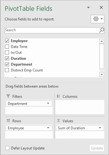
Starting on the Data sheet, you can go to the Insert tab and choose Pivot Table, inserting it on a new sheet. On the Pivot Tables pane, just move Employee to the Rows area. Then move Duration to the Values area and Department to the Filters area.

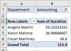
This creates a table that can be filtered down by department. As you select the department you want, it automatically changes to list the employees in that department and the total duration of their work hours. This is how the Accounting Department would look, for example:

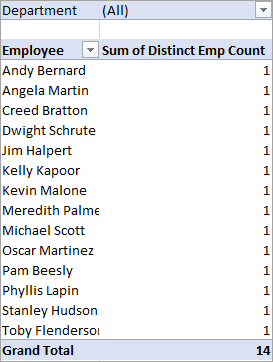
Another metric on the dashboard that we need to calculate is average number of hours per department. To accomplish this, we can duplicate the pivot table we've already created and swap out Duration for Distinct Employee Count.

This will give us a pivot table that looks like this:

Adding a Slicer

Now that we have these two pivot tables, we want to tie them together so that if we filter by department on one of them, the filter automatically applies on the other. We can do this by adding a slicer to the worksheet.

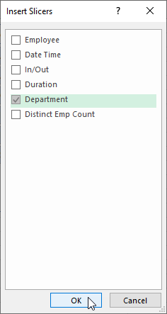
To add a slicer, start from anywhere in either of the pivot tables and go to the Pivot Table Analyze tab. Choose Insert Slicer, and then check the box for Department. Click OK.

That will create your slicer. If you right-click on your slicer, you can then choose Report Connections on the menu that appears. This will allow you to connect the pivot tables through the slicer. Just make sure both check boxes are selected for the pivot tables and hit OK.

To calculate the average number of hours per department, we just divide the Grand Total for the hours table by the Grand Total for the employee count table.

When we do this, Excel automatically populates the formula with the GETPIVOTDATA function because it is pulling from the pivot tables. The formula looks like this:

This returns a dynamic average calculation that changes as the pivot table is filtered.

Icons with Conditional Formatting

To create icons that appear to be semi-transparent or have a grayed-out look, I've simply set up a Shapes worksheet. This sheet has a couple of cells formatted with white fill and a 15% transparency. (These settings can be found on the Format Shapes Pane, accessed through the right-click menu or by typing Ctrl + 1).

These formatted cells will be overlaid on icons of your choosing. I found my icons at iconfinder.com.

Essentially, I've set up a formula that indexes a different named range depending on whether the department's hours are more than or less than the goal. (Click here to learn more about the INDEX function.) Those named ranges will display a shape that either has no formatting, or the slightly transparent formatting that I mentioned above.

This overlaid transparent shape makes the icon obscure but still visible, so it gives a grayed-out appearance.

See my note and additional file in the Downloads section at the top of the page about using two different colored icons instead of the transparent shape for Excel 2010.

There are also text boxes under the icons that are used to display the numbers.  These are linked to the corresponding cells with a formula that returns the average depending on whether or not it is less than or more than the goal amount.

Conclusion

While I love the newest features and functions that the latest version of Excel bring, it's great to see how we can solve this problem with some of the older tools in our Excel toolbox.  There are always so many ways to solve the same problem in Excel, so if you have any other ideas or suggestions, I'd love to hear them. Just leave a comment below.