Bottom line: Learn how to use the COUNTIF function instead of VLOOKUP to determine if a value exists in a list or range.
Skill level: Beginner
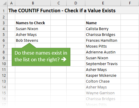
Problem – I want to check and see if the names in column B exist in this long list of names in column E.
There are a lot of different ways we can solve this problem with formulas in Excel. You might be inclined to use a VLOOKUP formula, and that would work just fine.
However, there are a few advantages to using the COUNTIF function instead.
- It's faster
- Easier
- And less prone to errors.
So let's learn how COUNTIF works.
Video Tutorial on How to Use COUNTIF
Here is a video from The Ultimate Lookup Formulas Course that explains how to use COUNTIF instead of VLOOKUP.
*Double-click the video to watch full screen.
There are over 100 short videos just like the one above included in the Ultimate Lookup Formulas Course.
This course has been designed to help you master Excel's most important functions and formulas in an easy step-by-step manner.
The Ultimate Lookup Formulas Course is now part of our comprehensive Elevate Excel Training Program.
Click Here to Learn More About the Elevate Excel
Download the Example File
Download the Excel file to follow along.
The COUNTIF Function Explained
COUNTIF is a very simple function. It's job is to search a range for a value and tell you how many cells match that value.
In the example below I am using a COUNTIF function to return the number of times the word “Surf” exists in the range. The result is 3.

Arguments: COUNTIF only has two arguments (Range, Criteria).
- Range – this is the range we want to search for the lookup value (Criteria).
- Criteria – this is the value we want to find.
Rules: By default COUNTIF is going to look for an exact match of each cell's entire value. You can add wild cards and conditional/relational operators to the criteria to look for partial matches.
Result: COUNTIF returns a numerical value for the number of cells that matched the criteria in the range. If the COUNTIF returns a number greater than or equal to 1, then that means the value exists in the list. If COUNTIF returns a zero then there are no cells that match the criteria.
So back to our original problem, we can use COUNTIF to see how many times the names exist in the list.
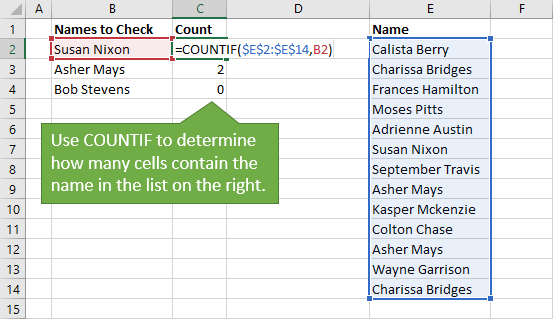
The cells in C2:C4 contain the COUNTIF function.
When COUNTIF returns a zero (0) this means the value does not exist. So the result in cell C4 tells us that the name Bob Stevens does not exist in the list.
Why Use COUNTIF Instead of VLOOKUP?
When you just want to determine if a value exists in a list then I recommend using COUNTIF over VLOOKUP. It has a few advantages that make it more efficient, and also give you more insight to your data.
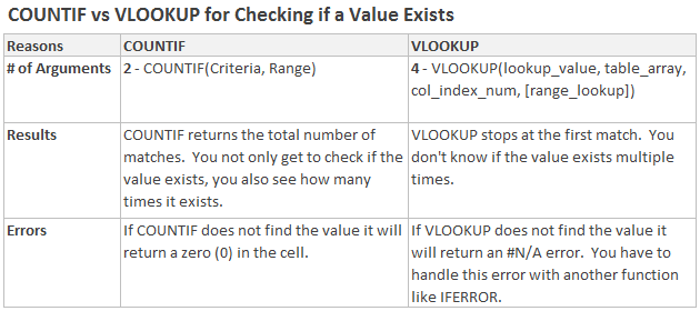
Here are 3 reasons to use COUNTIF instead of VLOOKUP (when you just want to see if a value exists in a range of cells):
- The COUNTIF function only has two arguments making it really fast and easy to write the formula. VLOOKUP has four arguments.
- COUNTIF returns the total number of matching values in the range, so you can see if there is more than one matching value. VLOOKUP cannot do this, it only returns the first match.
- If the value does not exist, COUNTIF will return a zero (0). You do not need to worry about a formula error. With VLOOKUP, the formula would return an error and you would use and error handling function like IFERROR to handle the error.
Here is a comparison table of the list above, just in case your boss asks why… 🙂
Checkout my article on VLOOKUP Explained at Starbucks if you want to learn more about how the function works.
COUNTIF vs VLOOKUP for Determining If A Value Exists
Here is an example of solving the same problem with COUNTIF vs VLOOKUP.
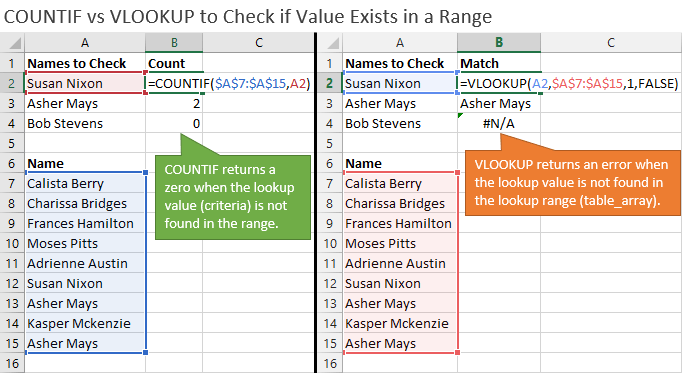
The COUNTIF returns a number greater than or equal to 1 if the value exists in the list. It returns a zero if the value does not exist.
The VLOOKUP formula is going to return the matching value from the list. VLOOKUP returns a #N/A error if it can't find the value in the list.
Obviously the VLOOKUP formula is longer, more complex, and will take more time to write.
Don’t Forget About COUNTIFS
The COUNTIF function has a big brother named COUNTIFS. This function allows you to specify multiple criteria in multiple ranges. You could use it to answer the question of how many Bob's are in the East region from the data set below.
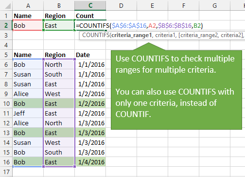
=COUNTIFS(criteria_range1, criteria1, criteria_range2, criteria2, …)
You can add up to 127 criteria!
You can also use COUNTIFS with only one criteria, just like you do with COUNTIF.
That means you could use COUNTIFS all the time instead of COUNTIF. I know a lot of people do this and that is perfectly fine. I wanted to keep it simple by explaining COUNTIF first.
So now you know two new functions that you can use instead of VLOOKUP to find a matching value!
Please leave a comment below with any questions.
Get More Training
This video and lesson are from The Ultimate Lookup Formulas Course. There are over 100 short videos just like the one above included in this self-paced online course.
This course has been designed to help you master Excel's most important functions and formulas in an easy step-by-step manner.
The Ultimate Lookup Formulas Course is now part of our comprehensive Elevate Excel Training Program.


Hi Jon,
This is excellent. I will use COUNTIFS instead of COUNTIF and replace VLOOKUP wherever possible. Great help.
Thanks Sastry! I am happy to hear it helped. Have a great day! 🙂
Really helpful.God bless
Thanks Rahul! 🙂
Hi. In the past, it has always been necessary to ensure that the the two criteria ranges when using =COUNTIFS have to be of exactly the same number of rows. Is this still the case now?
Regards,
Colin
Hi Colin,
Yes that is still the case. Your criteria ranges will need to be the same number of rows or columns. They don’t necessarily need to start and end at the same row or column, but they do need to contain the same number of rows or columns. Let me know if you have any questions. Thanks!
Is it possible to use COUNTIFS with the same range and just multi[le criteria?
Thanks
Great question Aimee. You can use COUNTIFS for multiple criteria in the same range, but it takes a few extra steps to make it work. There are basically two options.
1. You can use two separate COUNTIFS functions and add them together. =COUNTIFS(criteria1) + COUNTIFS(criteria2). This would count each criteria on the range individually then sum them up.
2. You can wrap the COUNTIFS in a SUM formula and add both criteria in curly brackets to create an array. =SUM(COUNTIFS(criteria_range, {criteria1,criteria2})
Here is an article that explains both solutions in more detail.
http://excelxor.com/2014/09/28/countifs-multiple-or-criteria-for-one-or-two-criteria_ranges/
Thanks!
Thanks Jon. That is helpful.
I need to know can I do to use the countif function using the vlookup to select different range with the same criteria, for instance: =countif(vlookup(A1,data,2,false),”X”).
This way I will be able to count the same criteria in different range with the need to create a formula for each one of the ranges.
I tried to do use it this way but it gives me an error, can you help me please, thanks in advance.
Hi Robert,
Great question! You can use the INDEX function for this. INDEX will return an array and you can specify the column number you want to look at. The formula will look something like the following.
=COUNTIF(INDEX(data,,1),”X”)
The 1 represents the column number, which is the 1st column of the “data” range. If you changed that to 2 it would look in the 2nd column. You can also change the 1 to reference a cell that contains the number. Or you can use the MATCH function if you want to lookup the column header name to return the column number back to the INDEX function.
I also have a free video series on the lookup formulas that covers VLOOKUP, INDEX/MATCH, and more.
I hope that helps.
Hello, great site so congrats for that, very helpful
I have used countifs to know how many securities match certain criterias such as spread, maturity etc
However while it does give me a number, i am helpless to design a fomrula allowing me to identify which securities are a match and counted by the Countifs formula
Is there an easy way to get the cells that are a match on top of just their number?
Thanks a lot
In column 3 (last spreadsheet shown here) are pipe size. Last column is length of each pipe size. I’m looking for formula that will add length of each pipe size. There are multiple lines consisting of the same pipe size so I’m looking for vlookup, match index showing accumulative total in single cell below.
SIZE GRAND TOTAL LENGTH (FT)
HSS10X8X1/2 ?
HSS10X8X3/8 ?
HSS10X8X5/8 ?
HSS6X6X1/4 ?
HSS8X8X1/2 ?
L3X3X1/4 ?
L3X3X3/8 ?
L4X4X3/8 ?
L6X4X3/8 ?
QNTY PIECE MARK SIZE DESCRIPTION LENGTH LENGTH TOTAL LENGTH (FT)
FT IN FT
2 17C2 HSS8X8X1/2 COLUMN 18.00 6.50 18.54 37.08
2 17C2 HSS10X8X1/2 BEAM 0.00 2.00 0.17 0.33
1 17C3 HSS8X8X1/2 COLUMN 7.00 2.25 7.19 7.19
1 17C3 HSS10X8X3/8 BEAM 0.00 2.00 0.17 0.17
1 18C1 HSS8X8X1/2 COLUMN 18.00 5.31 18.44 18.44
1 18C1 HSS10X8X5/8 BEAM 0.00 2.25 0.19 0.19
1 18C1 HSS6X6X1/4 BEAM 4.00 3.88 4.32 4.32
2 19C1 HSS8X8X1/2 COLUMN 18.00 6.50 18.54 37.08
2 19C1 HSS10X8X1/2 BEAM 0.00 2.25 0.19 0.38
4 19C1 HSS6X6X1/4 BEAM 4.00 3.88 4.32 17.29
1 19C2 HSS8X8X1/2 COLUMN 7.00 2.25 7.19 7.19
1 19C2 HSS10X8X3/8 BEAM 0.00 2.25 0.19 0.19
1 20C1 HSS8X8X1/2 COLUMN 17.00 6.00 17.50 17.50
1 20C1 HSS10X8X1/2 BEAM 2.00 5.25 2.44 2.44
1 20C2 HSS8X8X1/2 COLUMN 17.00 6.00 17.50 17.50
1 20C2 HSS10X8X1/2 BEAM 0.00 2.25 0.19 0.19
1 21C1 HSS8X8X1/2 COLUMN 18.00 6.50 18.54 18.54
1 21C1 HSS10X8X1/2 BEAM 0.00 5.50 0.46 0.46
1 21C2 HSS8X8X1/2 COLUMN 7.00 2.25 7.19 7.19
1 21C2 HSS10X8X3/8 BEAM 0.00 5.50 0.46 0.46
1 22C1 HSS8X8X1/2 COLUMN 17.00 6.00 17.50 17.50
1 22C1 HSS10X8X1/2 BEAM 2.00 5.25 2.44 2.44
1 22C2 HSS8X8X1/2 COLUMN 18.00 6.50 18.54 18.54
1 22C2 HSS10X8X1/2 BEAM 0.00 5.50 0.46 0.46
1 23C1 HSS8X8X1/2 COLUMN 7.00 2.25 7.19 7.19
1 23C1 HSS10X8X3/8 BEAM 0.00 5.50 0.46 0.46
1 23C2 HSS8X8X1/2 COLUMN 7.00 2.25 7.19 7.19
1 23C2 HSS10X8X3/8 BEAM 0.00 2.25 0.19 0.19
Hello,
I am looking for assistance with coming up with a function that would return a value from a range b/n two numbers:
Price: $0.00-$2.25 $2.26-$2.99
Year 1 $40,500 $45,700
Year 2 $30,400 $35,500
From the example above, if a given price is b/n $0.00-$2.25 and I need value for Year 1, I need the function to return $40,500.
I would greatly appreciate any input.
Thank you,
George
How we can use COUNTIF and VLOOKUP formula together?
Just wondering if you got your answer and if you can share?
Hello,
I’m trying to use =countif to identify a smaller set within a larger set, and be able to filter by it. Why I drag my copy/fill box down with my =countif formula, it is auto shifting the range down as well. I want the criteria to shift down, but not the range. HOw do I keep this from shifting?
Thanks!
I have a spreadsheet where we are scanning in multiple carton numbers as text. All carton numbers are 20 characters long. They either start with 000 or 999. The cartons beginning in 000 will all return the correct value when doing a count if and looking for a specific carton in a data drop sheet. The problem I have is when I look for a carton starting with 999 it returns a value of all 7095 cartons that begin with 999. Is there a way around this that I am not seeing?
Great post! I never realized how versatile the COUNTIF function could be as an alternative to VLOOKUP. The video definitely helped clarify the process. Thanks for sharing these tips!
This post is a game changer! I always relied on VLOOKUP for my data analysis, but using COUNTIF seems so much more efficient for certain tasks. The video explanation was also super helpful—thanks for breaking it down! Can’t wait to try this in my next project.
Great post! I never realized how powerful the COUNTIF function could be as an alternative to VLOOKUP. The video was really helpful in demonstrating the process. Thanks for sharing these insights!
Great post! I always relied on VLOOKUP, but your introduction to the COUNTIF function really opened my eyes to a more efficient way to analyze my data. The video was super helpful too—thanks for breaking it down so clearly!
Great post! I never thought about using COUNTIF as an alternative to VLOOKUP. The video was super helpful in illustrating how it works. Can’t wait to try this out in my spreadsheets!
Great post! I never realized how versatile the COUNTIF function could be compared to VLOOKUP. The video made it super clear, and I can’t wait to apply this in my spreadsheets. Thanks for sharing these tips!
Great tips on using the COUNTIF function! I never thought about using it instead of VLOOKUP for counting occurrences. The video was super helpful for visualizing the process. Thanks for sharing!
Great post! I never thought about using COUNTIF as an alternative to VLOOKUP. The video explanation really clarified how to implement it effectively. Thanks for sharing this valuable insight!
Great post! The COUNTIF function seems like a powerful alternative to VLOOKUP for specific use cases. I love the video explanation too; it made the concept much clearer. Thanks for sharing these insights!
Great post! I always thought VLOOKUP was the go-to for counting criteria, but your explanation of using COUNTIF is a game changer. The video really helped clarify the steps too. Thanks for sharing!
Great post! I never realized how easily the COUNTIF function could replace VLOOKUP for certain tasks. The video was especially helpful in illustrating your points. Can’t wait to apply this in my spreadsheets!
Great post! I never thought about using COUNTIF as an alternative to VLOOKUP. The video was incredibly helpful too. I’m excited to try it out in my spreadsheets! Thanks for sharing!
Great post! I never thought about using COUNTIF as an alternative to VLOOKUP. The video really helped clarify the process. Can’t wait to try this out in my own spreadsheets! Thank you for sharing!
This was such a helpful post! I never thought to use COUNTIF in place of VLOOKUP. The video made it all so clear—thanks for breaking it down!
Great post! I never realized how much simpler counting unique values could be with COUNTIF compared to VLOOKUP. The video was super helpful—thanks for breaking it down so clearly! Can’t wait to apply this in my spreadsheets.
Great post! I never thought to use COUNTIF as an alternative to VLOOKUP. The examples you provided made it really clear. Thanks for sharing the video as well—super helpful!
This was an incredibly helpful post! I’ve always relied on VLOOKUP for my searches, but using COUNTIF seems so much more efficient for my needs. The video really clarified the steps—thank you for breaking it down so clearly! Can’t wait to try it out in my next project.