Bottom Line: Learn how to use the XOR function in Excel to analyze attendance data.
Skill Level: Intermediate
Download the Excel File
The file that I work within the video can be found below. You can use it to follow along and reconstruct what I'm doing in the video.
Compatibility: This file uses the new Dynamic Array Functions that are only available on the latest version of Office 365. This includes both the desktop and web app versions of Excel.
I'm planning to post a bonus episode in this series that covers how to make the dashboard with older versions of Excel using pivot tables instead.
Part of a Series
Just so you have some context, this post is the first of six in a series that resulted from an Excel Hash competition. Each year, Excel geeks like myself are tasked with building a worksheet that contains specific features. We compete to see whose solution is best. It's a lot of fun.
My entry from this year is a salute to one of my favorite shows, The Office. It's a dashboard that takes simple timestamp data and turns it into an attendance reporting tool that Dwight Schrute could proudly use to police his fellow coworkers.
If you'd like to see my entry for this year, watch this: Excel Hash: Attendance Report with Storm Clouds & Fireworks.
Here are the other posts in the series:
- How to Use the XOR Function (this post)
- How to Use XLOOKUP for Reverse Order Search
- Return Multiple Values for a Lookup Formula in Excel with FILTER and UNIQUE
- How to Sort with a Formula in Excel Using SORT and SORTBY Functions
- How to Create a Dynamic Drop-down List that Automatically Expands
- How to Create Icons with Conditional Formatting in Excel
Bonus: How to Create the Dashboard that is compatible with All Versions of Excel
The XOR Function
Our first step in creating this attendance dashboard is to take all of the timestamp data and determine if each entry is an “In” or “Out” entry.
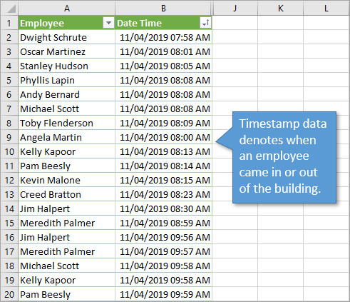
The logic is fairly straightforward. If there is one entry for any given employee, it means that they have come in to work and haven't yet left. A second entry would indicate that they are now out of the office. So what we are really looking for, initially, is to know if there are an odd or an even amount of entries in the running list. That way, we can label the employee “In” or “Out” of the office.
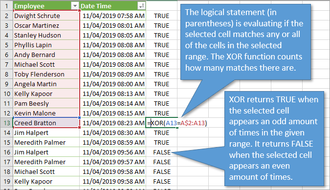
That's where the XOR function comes in. This function returns a TRUE result if there is an odd number of TRUE results in a range. Likewise, it returns FALSE if there is an even amount.
Note: For the purposes of our attendance tracker, the data should be sorted into chronological order.
Compatibility: The XOR function is available in Excel 2013 and later. If you have an older version you can use the ISODD(COUNTIF()) formula that I explain in the video and below.
Writing the XOR Function
To use the XOR function, simply type =XOR and Excel will prompt you to enter logical statements. You can also just feed it an array of true/false values.
For example in the video, the reference range that we want is (A2=A$2:A2). This tells Excel to return TRUE if the name in cell A2 is the same as any of the names found in the range from A2 to A2. Of course, that is only one cell, but as the formula is copied down to the cells below it, the range automatically expands. (The beginning of the range will always remain A2 because of the absolute reference (dollar sign), while the end of the range will change.)
The XOR function essentially evaluates how many times the selected cell matches the entries in the selected range. It returns TRUE when there is an odd amount and FALSE when even.
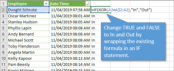
To make the report more understandable, we can wrap the function in an IF statement. If the function returns TRUE, the cell can read “In” and if FALSE, it can say “Out.”
So the final formula would be =IF(XOR(A2=A$2:A2),”In”,”Out”)
Using Table Range References
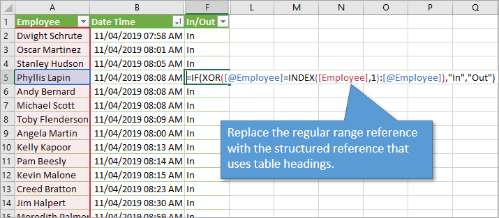
One quirk with Excel is that if you use the range references as I've outlined above (A$2:A2), it may not automatically extend when you add data to the bottom of your range. So an alternative is to use table range references.
Using INDEX, we can compare the first cell in a column with a range of cells from that same column. This accomplishes the same thing we did above with the regular range reference.
With our table reference, our range would be replaced with ([Employee]=INDEX([Employee],1):[@Employee]). This may look a bit gnarly if it's the first time you've dealt with the INDEX function. However, using this option is much better if data is continually being added to your report.
Conclusion
If you don't want to use the XOR function, you can use a combination of COUNTIF and ISODD as an alternative.
It would look like this: =ISODD(COUNTIF(A$2:A2,A2))
See the video above for details about how to construct that.
The next video in the series will take a look at calculating the duration of time that the employees were in the office.
I hope this post was helpful in explaining how the XOR function works. Please leave a comment below if you have questions about it.


Congratulations Jon for winning the Excel hash competition, your solution is awesome and demonstrates a clever use of infrequent functions, great!!
It’s the first time I hear about the XOR function, Excel never stops with surprises, wow!
I have a question about using table references, why was the Index function used?
Great video! Is there any calculation speed difference between the XOR method vs. the ISODD(COUNTIF ) method. Also are structured references faster than cell references. I agree that the structured reference looks more confusing, and would rather avoid them if sharing the workbook.
Hey Rich,
Great questions!
I have not done speed tests on either. My hunch is that COUNTIF might be faster but I could be wrong.
The structured references are going to be more bulletproof if you are adding rows to the table with that running total reference. The regular references with mixed absolute/relative references don’t always expand well in Tables.
I hope that helps. Thanks again and have a nice day! 🙂
Hi John,
First, congratulations on winning the competition.
Secondly, the XOR function isn’t available on all Excel versions.
Can you please specify which versions have it?
Best Regards,
Meni Porat
Thank you, Meni! I added a compatibility section above. XOR is available on Excel 2013 and later. On older versions, you can use ISODD(COUNTIF()) instead. I explain that in the video and article as well.
Thanks again and have a nice day! 🙂
I had the same question, except I found that control-shift-enter makes it work as with other array functions I’ve used. But I also noted that many of your functions in the workbook are for future functionality not yet on my version of O365. Curious about what they are (since we are only on Video 1), but also when they might be available to a wider audience. Thank you for all of your videos. I learn something with each of them.
Hi Terry,
Sorry, I should have made that more clear. The formulas use the functionality of the new Dynamic Array Formula update for Office 365 subscribers. The features are currently being rolled out to subscribers, but it does depend on which channel you are on. Currently you will have to be on the Monthly channel to get the latest updates.
Here is a post and video that explains more about Dynamic Arrays.
https://www.excelcampus.com/functions/dynamic-array-formulas-spill-ranges/
I hope that helps. Thanks again and have a nice day! 🙂
Hi Jon,
Can you re-post example workbook? It keeps crashing when I try to open it.
Thanks,
Colin
Hey Colin,
I’m sorry to hear that. I just reposted two files. One is the “follow along” version with the data only. The second is the final file.
It doesn’t crash for me. However, it could be a compatibility issue. If you are on an older verison of Excel there could be an issue with the new Dynamic Array Functions that are being used in this file.
You should still be able to open files with DA functions in older versions even though the formulas won’t work. Microsoft is slowly releasing the DA features and still working out the bugs.
I hope that helps. Thanks again and have a nice day! 🙂
Hi,
Here is a parsed example from the workbook. For some reason, I’m returning TRUE even when a repeat name is present?
Dwight Schrute TRUE =XOR(A1=A$1:A1)
Oscar Martinez TRUE =XOR(A2=A$1:A2)
Phyllis Lapin TRUE =XOR(A3=A$1:A3)
Dwight Schrute TRUE =XOR(A4=A$1:A4)
The formula should be array-entered, with Ctrl+Shift+Enter
Thanks Debra! 🙂
thanks a lot Debra ! i was encountering the same issue than Colin !!! and it does work now !! awesome !
Hi Colin,
Those are the correct results. You won’t start getting FALSE values until row 16. The running total reference A$1:A2 is only looking for duplicates in the current row and ABOVE. Not in the rows below.
Was always in a little bit of confusion in regards to XOR function, this has helped me a lot. I will make sure to practice this all over again.
Thank you Rishi! 🙂
A very good job, Jon .
Thanks for sharing .
Hello Jon,
Thank you for this video of XOR function.
I copied the name list as in your example to my Excel in my computer then typed this function below
=XOR(A4=$A$1:A4)
The function doesn’t seem to check through all the array values that it ends up giving TRUE although some names appear more than once in the array list.
Do you know what was the issue?
Am using Microsoft Office Home 2019.
Got it! It appears that someone else had posted the same question before and someone else had given a reply on that. Thank you
I am just getting to review your dashboard series. I looked at the XOR Function, lesson 1. I downloaded the file and the final file. After watching the video I tried creating the formulas in the file but I had a problem.
As long as I used the cell reference, A2, both the ISODD XOR and the COUNTIF formulas worked fine. My problem is with the formula using the @EMPLOYEE. When I enter the formula pointing to cell A2 I get tblData[@EMPLOYEE]. When I copy the formula down it give me the result but the formula does not adjust for each name. Here is the formula as it comes into Excel:
=IF(XOR(tblData[@Employee]=INDEX(tblData[@Employee],1):tblData[@Employee]),”In”,”Out”).
When I remove the tblData portion the formula does not work at all. I went to Options, Formulas, and turned off formula reference. At this setting it just gives me the cell address, A2, when I point to it.
What am I doing incorrectly?
I used column I for the @EMPLOYEE formula (all filled in with IN), column J for the ISODD, COUNTIF formula (all filled in with IN and OUT) and K for the XOR formula (all filled in with TRUE and FALSE).
Also, the formulas did not automatically fill for each employee, I had to copy them down.
I tried using the Ctrl+Shift+Enter to put the curly braces around the formula and it still did not work for the @EMPLOYEE formula.
Thank you for your assistance in resolving my question.
Howard