Return Multiple Values for a Lookup Formula in Excel with FILTER and UNIQUE

Bottom Line: Learn how to use the FILTER and UNIQUE functions to return multiple values for a lookup based on a condition.

Skill Level: Intermediate

Download the Excel File

The file that I work within the video can be found below.  You can also download the “Follow Along” version if you'd like to practice building out the report.

Compatibility: This file uses the new Dynamic Array Functions that are only available on the latest version of Office 365. This includes both the desktop and web app versions of Excel.

I'm planning to post a bonus episode in this series that covers how to make the dashboard with older versions of Excel using pivot tables instead.

Building an Attendance Dashboard

This post is part 3 of a six-part series explaining how to build an interactive dashboard for attendance.  This attendance report was an entry for the Excel Hash competition.  

Here are the other posts in the series:

Dynamic Array Functions

This post will feature two of the new Dynamic Array Functions available through Office 365.  Dynamic Array Functions allow for multiple values to be to a range.  This is referred to as the Spill Range because the results spill over into blank cells beneath the cell that contains the formula.

This new functionality is really helpful, as you will see. The two Dynamic Array Functions we will be looking at in today's post are UNIQUE and FILTER. 

The UNIQUE Function

The UNIQUE function evaluates a range of data and pulls out all the duplicates, returning a list of unique entries from that range.

The function has three arguments, but only the first one is required. It is the Range/Array to evaluate.

In this example we want to create a list of unique employee names from our data table.  This will be used for the summary report of total duration per employee.

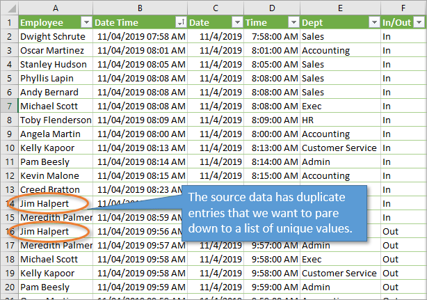
The data table contains a list of time entries with multiple rows per employee.  So in order to return a list of unique values we can use the following formula.

=UNIQUE(tblData[Employee])

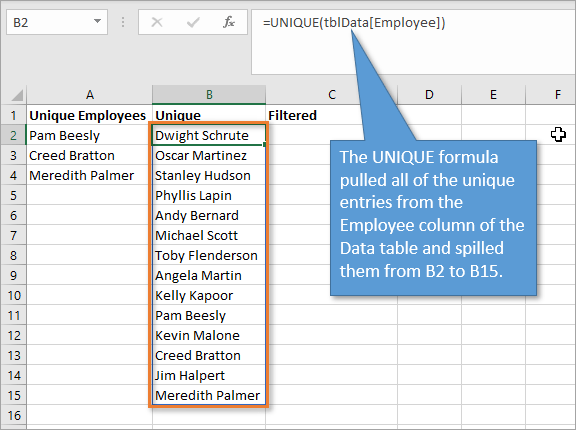
The result is a list of all employees in the data set.

The FILTER Function

Now we want to filter our list of employees by department.  The FILTER function is great for this task.  It is essentially like a lookup that returns multiple results.  We want to lookup the a specific department in the department column and return all the matching employee names (people in the department).

The FILTER function has three arguments. The first is the array that we want to return. As before, this is the Employee column on the Data sheet.

The second argument is Include, and it is the filter criteria that we want to specify. In our case, that criteria is the department. So our argument will essentially tell Excel to examine the list of departments on the Data tab and see which ones match the department that's in our dashboard drop-down list.

Dashboard!B5=tblData[Dept]

The third argument [is_empty] indicates what to do if no matches are found.  FILTER has built-in error handling so the formula will not return an error if nothing matches the filter criteria.  I used the word “Empty”, but you can use a more descriptive phrase if other people are using your file.

Our final formula, then, looks like this:

=FILTER(tblData[Employee],Dashboard!B5=tblData[Dept],”Empty”)

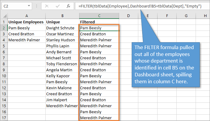
The formula returns a list of all the employees in the specified department.  As you can see in the image above, there are duplicates that we need to eliminate.

Combining the Functions

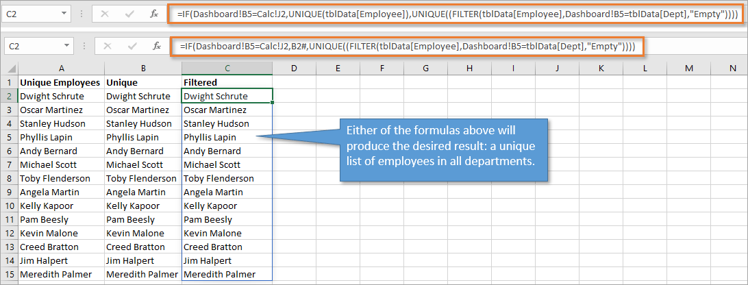
Because the FILTER function returns duplicate entries, we can combine it with UNIQUE to pull those out:

=UNIQUE(FILTER(tblData[Employee],Dashboard!B5=tblData[Dept],”Empty”))

Filtering for All Departments

The last problem to overcome is filtering by all departments. Because “All Depts” is not listed for any employee specifically, the filter function cannot find it, and the word “Empty” is returned when that option is selected on the dashboard.

To take care of this, we can wrap everything we have done so far (represented by XXX below) in an IF function.

=IF(Dashboard!B5=Calc!J2, UNIQUE(tblData[Employee]),XXX)

Because we have already pulled out a unique list of employees, an alternative would be to reference that spill range, which is B2#.

=IF(Dashboard!B5=Calc!J2, B2#,XXX)

Conclusion

Using these Dynamic Array Functions is a really neat way to quickly return multiple results to multiple cells. They are a great alternative to VLOOKUP and allow you to create a dynamic range based on a certain criteria.

UNIQUE removes duplicates in a list, returning a clean list of unique values.  FILTER returns multiple results based on lookup criteria with a simple straightforward formula.

If you have questions about this post, I invite you to ask them in the comments below.