New Excel Features: Dynamic Array Formulas & Spill Ranges

Bottom Line: Learn about the new Dynamic Array functions and formulas that will eventually replace the Ctrl+Shift+Enter array formulas.

Skill Level: Beginner

Video Tutorial

Download the Excel File

Here's the file I use in the video. Unfortunately, these functions are only available to a portion of users on Microsoft's Office Insiders Program.  So you might not have access just yet.  The Insiders program is free for all Office 365 subscribers and gives you access to early release builds and features.

Dynamic Array Functions & Formulas

Microsoft just announced a new feature for Excel that will change the way we work with formulas.  The new dynamic array formulas allow us to return multiple results to a range of cells based on one formula.  This is called the spill range, and I explain more about it below.

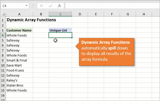
Excel currently has 7 new dynamic array functions, with more on the way.  We can use these to create a list of unique values (remove duplicates), sort a list, output a filtered range of data, and so much more.  Plus, existing functions can utilize this same spill range functionality.

Goodbye Ctrl+Shift+Enter

The goal of this new functionality is to eventually replace array formulas that we input with Ctrl+Shift+Enter (CSE).  Don't worry, that will be a long goodbye.

CSE formulas are much more complex, and we usually have to guess at how many cells we need to copy them to.  Here's a post and video where I explain more about them.

The image below shows a CSE array formula, enclosed in curly brackets, that can be used to create a list of unique values (remove duplicates).

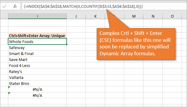
If you don't have the new functionality yet, checkout this post by my friend Dave at Exceljet on how to the CSE array formula to return unique values.

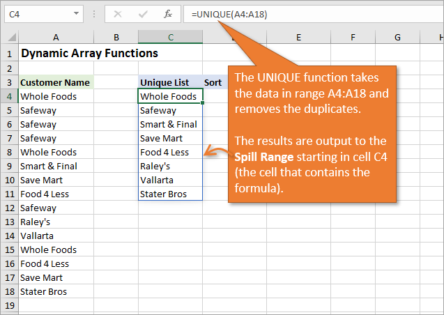
Let's take a look at how much easier this will be with the new dynamic array function, UNIQUE.

The UNIQUE Function in Excel

With the new UNIQUE function you'll be able to create a list of unique values (remove duplicate entries) using a very simple formula.

To create a list of unique values, you simply reference the range that contains duplicates in the array argument for UNIQUE.

When the formula is entered, the results will automatically spill down into the cells below.

The UNIQUE function has additional optional arguments as well:

• [by_col] – Allows you to compare by rows or columns when the array is multiple columns wide.  Default value is False, to compare by rows.
• [occurs_once] – Allows you to only return values that occur once in the array (range).  This is a great option.  Default value is False, to return all unique values.  Set it to True to return values that only occur once.

Here is the help page on the UNIQUE function to learn more about it.

For those who need to remove duplicates today and don't have the luxury of waiting for the UNIQUE function to roll out, here's a post that covers 3 ways to remove duplicates and create a list of unique values.

The Spill Range

Get used to the term “spill” for Excel.

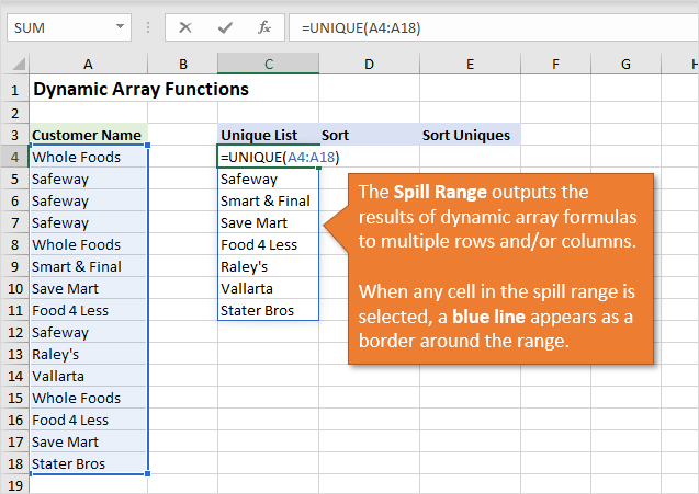
The range of cells that contains the results is called the spill range.  This range can be multiple rows and/or columns, as you'll see in the examples below.

The spill range is brand new functionality in Excel that will make our lives much easier.  Previously we had to use Ctrl+Shift+Enter array formulas, and try to guess how many cells to copy it to.

Excel is now going to do all that work for us!

When any cell in the spill range is selected, a blue line appears as a border around the range.  What happens if something is blocking the spill range?

#SPILL Error

If there is already data in the spill range, a #SPILL error will be returned.  This indicates that the range where the results need to spill down is not completely blank.

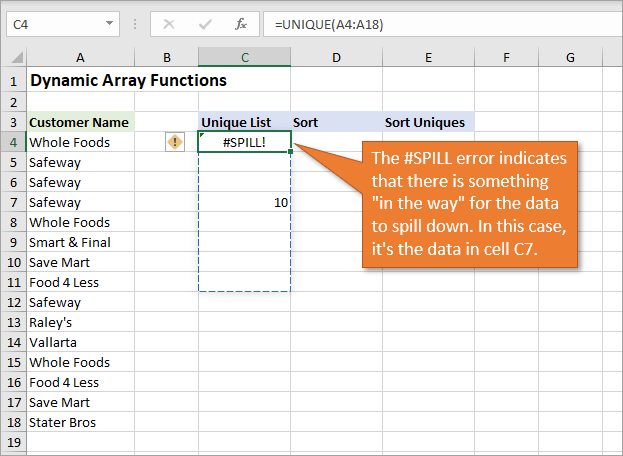
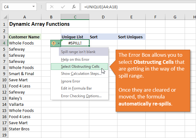
The error box appears and allows you to select the cells that are obstructing the spill range.  You can then move or delete those cells, and the formula will automatically re-spill.

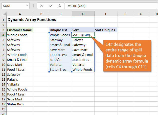
The SORT Function

SORT is another new and very useful function.  This outputs a sorted list of the array (range) specified in the function's first argument.

SORT has additional optional arguments for [sort_index], [sort_order], [by_col].  Here is the help page on the SORT function to learn more.

Spill Reference Notation – Spill Ref

In the example above you'll notice that I used C4# in the array argument for the SORT function.

This is referred to as a Spill Ref.  It allows us to create a reference to the entire spill range by placing a # (hashtag or pound symbol) after the address of the first cell in the spill range.

There are a few ways to create a spill ref:

• Type or select the first cell in a spill range to create a reference to that cell.  Then type the # after it.  You will see a bounding box appear around the spill range.
• The other way is to select all the cells in the spill range.  The spill ref will automatically be created.
• A quick keyboard shortcut for this is to select the first cell in the spill range, then hit Ctrl+Shift+Down Arrow to select all the cells.  This automatically creates the spill ref as well.

Uses for Spill Refs

Spill refs are extremely useful.  You can use them as the source range for other dynamic array formulas, as I did above with sorting the list of unique values.

You can also use them for regular formulas if you want to do a calculation (SUM, COUNT, etc.) or lookup (VLOOKUP, INDEX, MATCH) on the spill range.

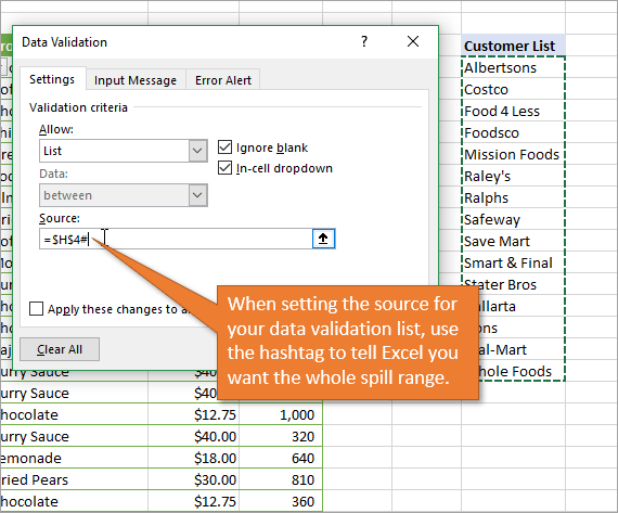
We can even use them for named ranges or data validation (example below).  Like I mentioned earlier, spill refs and spill ranges are terms we will use a lot in the future with Excel.

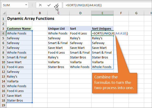
Combining Dynamic Array Functions

Dynamic array functions can also be combined in the same formula.  For example, we can use SORT and UNIQUE in the same formula to return a list of sorted unique values.

This is great for the source of a data validation (drop-down) list.

Using Dynamic Arrays for Data Validation Lists

These new formulas can also help to simplify Data Validation (or drop-down) lists in cells.

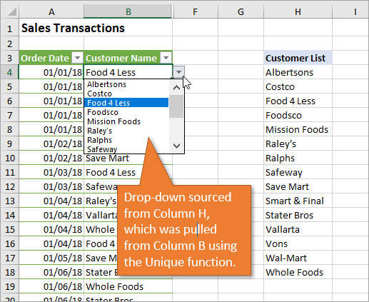
If you are not familiar with Data Validation lists, you can check out my post on the subject here. With this new formula, you can pull out the unique entries from a data set, just as above, and then use that new list as the source of your drop-down list.

In the example below,  I used the SORT(UNIQUE()) formula to create a list of uniques from Column B, and output it to Column H.  Then I use Column H as the source of my drop-down list for Customer Name.

To do this we can just use a spill ref to reference the spill range (H4#).  By adding the hashtag to the end, we are letting Excel know that we want the whole spill range, not just cell H4.

The amazing part is that the spill range automatically updates as items are added to column B.  Everything is dynamic, meaning we never need to do maintenance on our ranges or update our formulas.  The spill ref always includes everything in the automatically updating spill range.

Filter Function

FILTER is another great function coming to Excel.  With the Filter function we can use an entire table as the data source, and filter it down by one or multiple criteria.

For example, in the image below, I've filtered the data set on the left to just the information that applies to the customer Stater Bros (cell I1).  As I show in the video, the criteria cell(s) can be drop-downs to make for quick interactive reports.

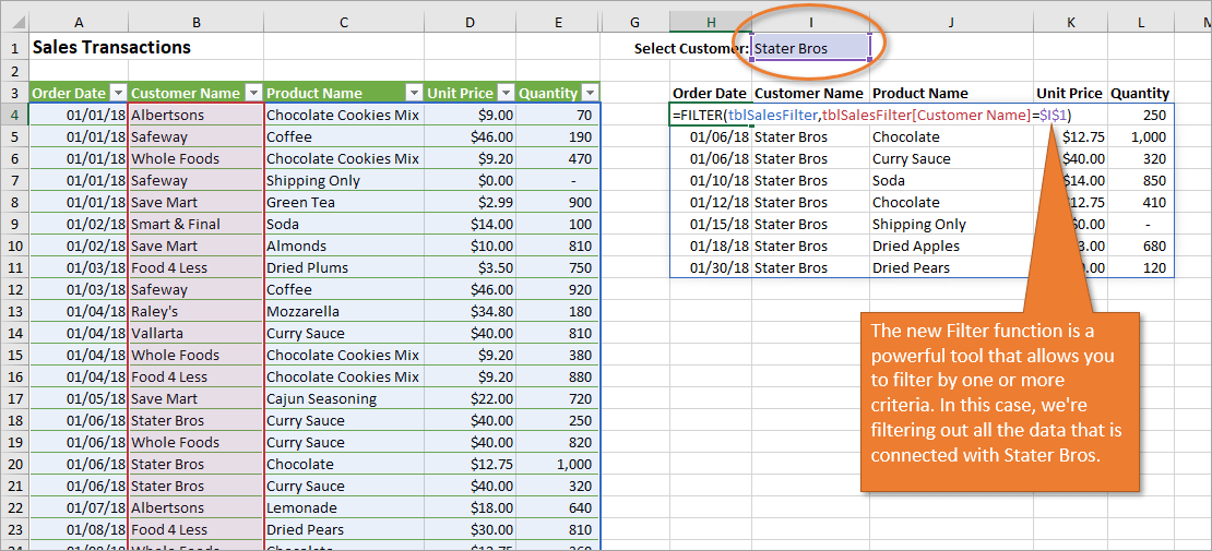
The goal of most array formulas is to do multiple calculations and return multiple results to a range of cells. This FILTER function really demonstrates how a lot can be done with just one simple formula. And again, since these these arrays are dynamic, the results will automatically be updated (re-spilled) any time changes are made to the source range or its precedents.

Dynamic Array Formulas Are Coming!

As I mentioned, these functions are not yet available to the general public.  The current availability is limited to a portion of users on Microsoft's Office Insiders Program (Insider channel).  The program is free for Office 365 subscribers.  There is no set release date to all Office 365 users yet, but hopefully that will be soon.

As of now, there are 7 new dynamic array functions:

• Filter – allows you to filter a range of data based on criteria you define.
• RandArray – returns an array of random numbers.
• Sequence – allows you to generate a list of sequential numbers in an array, such as 1, 2, 3, 4.
• Sort – sorts the contents of a range or array.
• SortBy – sorts based on the values in a corresponding range or array.
• Unique – returns a list of unique values in a list or range.
• Single – returns a single value at the intersection of a cell's row or column.  Update: The Single function has been removed from Excel and the @ symbol is now used instead for backward compatibility.

You can click any of the links above to read the Microsoft help article about each function.

Existing Functions Can Spill

You might be wondering about other existing array functions in Excel.  Well, those functions will spill too.  Here is an image of the model I used in my solution on the Dynamic Histogram Chart.

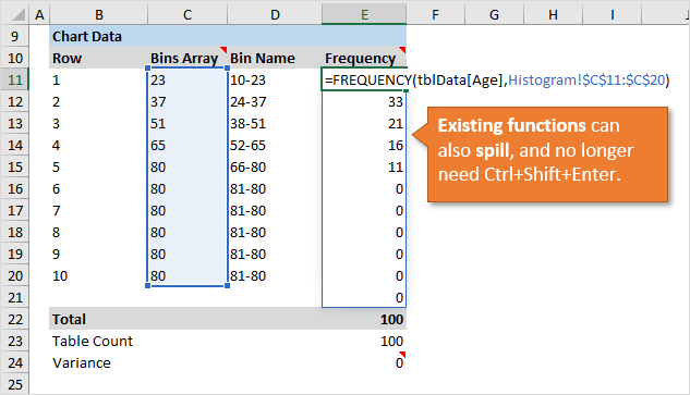
That solutions uses the FREQUENCY function.  In older versions of Excel we have to enter that formula with Ctrl+Shift+Enter and first select a range of cells for the output. I had to add extra rows to allow up to 10 bins.

However, with the new spill functionality that setup can actually be simplified.  I don't need all the extra rows with the max number starting in cell C16.  I could also use a spill ref for E11# to reference the dynamic range in a named range for the source of my chart.  Currently we can't use spill refs directly in charts, but I'm guessing that will be fixed.

So, the spill range is NOT limited to the new set of functions.  We are really getting two new features here: dynamic array functions and spill ranges.

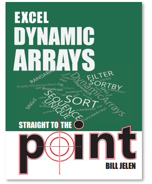
eBook on Dynamic Arrays

Another great resource to learn all about these functions before they release is a new eBook by Bill Jelen. It's called Excel Dynamic Arrays: Straight to the Point and it's completely free to download right now for a limited time. The promotional period has ended, but this is still a great resource at a very reasonable price.

Click here to get the eBook

Conclusion

I know, I know, what a jerk right?  I get to sit here and tease you about these new features that you probably can't use yet.

Dynamic arrays are coming soon though.  And I hope you're as excited as I am for this update.

If you have been using Google Sheets, then you know this isn't really new technology here.  However, Excel's implementation of the spill range and spill refs (A4#) is different (at the time of this writing).  It opens up a whole new world of possibility and simplicity with Excel formulas and other features.

You've probably heard me say, “there are always a million ways to solve the same problem in Excel…”  This new feature probably multiplies that number by another million, leaving us with a lot of new things to explore and learn in Excel. 🙂

I explain how to get these new features in the coming soon section above.

Are you excited for this?  Please leave a comment below and let us know.  Thank you!