Bottom Line: Learn to create dynamic data validation lists. These in-cell drop-down lists automatically expand to include new rows that are added to the source data range.
Skill Level: Intermediate
Video Tutorial
Download the Excel File
You can download the file I’m using in the video to practice on your own.
Dynamic Lists with Excel Tables and Named Ranges
Data Validation lists are drop-down lists in a cell that make it easy for users to input data. If you’ve never worked with data validation lists before, I suggest you start with this tutorial for creating drop-down lists in cells before moving on.
In today's post, I want to show you how to make your drop-down list dynamic. In other words, your list can automatically be updated with new options when you add or subtract entries to your source range.
This is done in three simple steps:
- Formatting the source range to be an Excel Table.
- Naming the range.
- Telling the Data Validation rules to pull the named range as your source.
I’ll explain in more detail below.
Step 1 – Format the Source Range as a Table
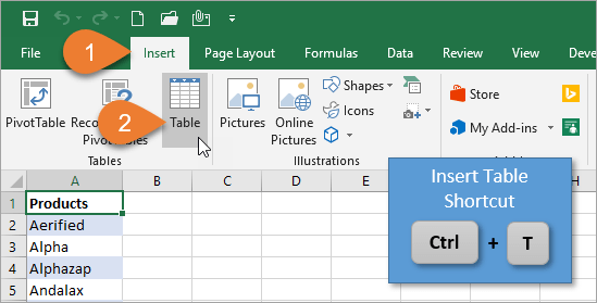
To begin, we will format our source range to be an Excel Table. On the Insert tab, you’ll chose the Table button. The keyboard shortcut for inserting a Table is Ctrl+T.
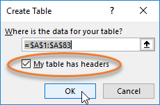
The Create Table window will appear, showing the range of cells that will be in your Table. Since our column begins with a header (“Products”), we want to make sure the checkbox that says “My table has headers” is checked. If we don't check that box, the column title will be included in our source range and will appear as one of the options in our drop-down list.
If you haven’t used Tables before, I recommend checking out my Excel Tables Tutorial Video.
Step 2 – Create the Named Range
The next step in our process is to name our range for the “Products” Table that we just created.
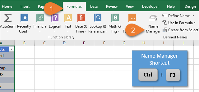
On the Formulas tab in the ribbon, you want to select the Name Manager (or you could use the the Ctrl+F3 keyboard shortcut instead).
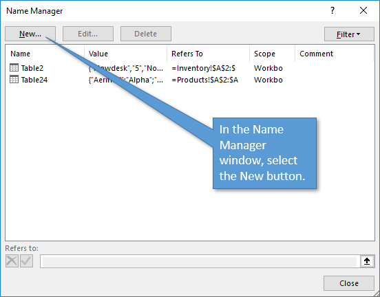
The Name Manager window will appear, and you will want to click on the New button.
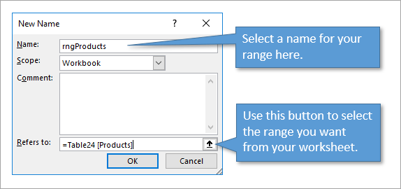
This brings up a new window that allows you to name your range. I like to prefix my ranges with “rng” to make them easier to find in formulas. However, the naming is completely up to you.
The “Refers to” field allows you to select the range that you want to include. The up arrow icon to the right of that field takes you to the worksheet. There you can highlight the selection that you want to use for your range.
Once you have defined your range, you can click OK, and then close the Name Manager window.
Step 3 – Reference the Named Range in the Data Validation Source
Now that we’ve named our range, we just need to tell that name to the Data Validation window so that it knows where to pull from for our drop-down list.
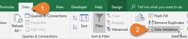
To do that, start with the cell that you want the drop-down list to be added to. Then access the Data Validation window by selecting the Data tab on the ribbon and clicking on the Data Validation button.
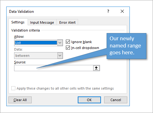
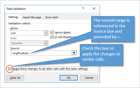
In the Data Validation window, under the Settings tab, we can type the name of our range into the Source field.
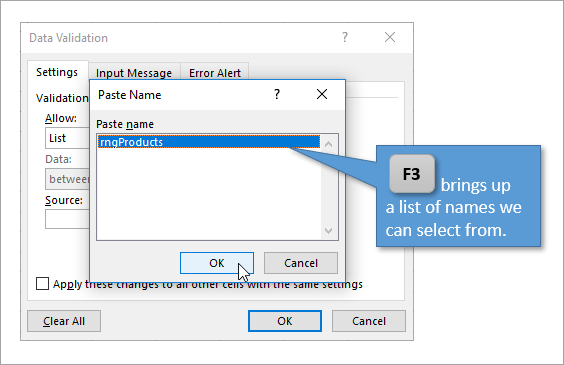
A shortcut to typing the name of our range is F3, which brings up a list of any ranges we’ve named. We can simply click on the range we want in order to select it.
Once you have selected the named range you want, click OK. But before leaving the Data Validation window, you want to check the checkbox that says “Apply these changes to other cells with the same settings.” This ensures that your drop-down list will be applied to similar cells in your worksheet.
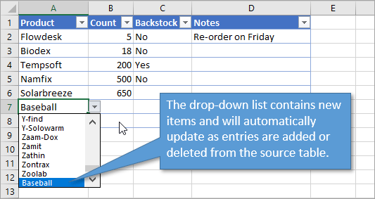
After we click OK, our drop-down list is now pulling from the Table that we have defined and named. So now any time you alter the Table, adding or deleting rows, the drop-down list will remain in sync with those changes.
Alternative to Named Ranges – INDIRECT
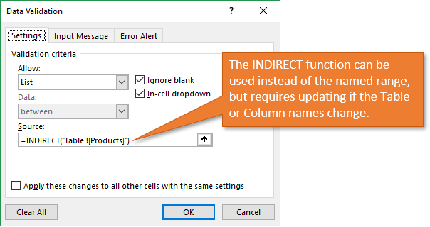
There are alternatives to using the named range in the data validation source. We can also use the INDIRECT function in the Source box, and reference the Table and Column name. The formula uses structured reference Table formulas, and looks like the following.
=INDIRECT("Table3[Products]")
You can type the formula directly in the source box in the Data Validation window. Just make sure the Table name and column name are correct.
I presented this technique in my article on dependent drop-down lists.
One drawback with the INDIRECT technique is that if you change the Table or Column names, the formula will NOT be updated. The drop-down button will still appear next to the cell, but you won't be able to click it.
Using the named range technique does allow you to change the name of the Table or Column. The reference in the named range will automatically be updated. Since multiple cells could be using this reference, it makes maintenance easier if you forget to press the “Apply these changes to other cells…” checkbox. Therefore, I recommend using the named range method described above.
Dynamic Data Validation Lists Save Time
By making your Data Validation lists dynamic, you don’t have to worry about updating your drop-down lists every time you make a change to your source data. This not only saves you time but hopefully adds a little peace of mind to your day. 😊
If you are interested in creating drop-down lists that are dependent on other drop-down lists, you can find out how to do that here. For example, if you choose Fruit in your first list, the options to choose from in your second list might be Banana, Apple, and Orange. But if you change your choice to Vegetable in your first list, the options in the second list change to Celery, Carrot, and Broccoli. This function is helpful if your lists drill down several levels or involve steps.
I've also created a free tool that helps you to search a data validation list, so you don't have to scroll through lots of entries to find the one you want. You can get that free search tool here.
I hope all of this information is helpful! If you have any questions about making your drop-down lists dynamic, please let me know in the comments below.


Hello sir,
I was working on excel workbook with vba it worked well on my PC it works but on other PC it doesn’t work
The error I get it’s
Catastrophic error then out of memory error
System Error &H8000FFF (-2147418113)
Please help
Hello,
I’ve found a simpler way with creating a named range.I still use a Table.
So instead of creating a named range for the validation list, in the field of the validation i write this simple formula =indirect(“myTable[theColumn]”)
Hi Miaousse,
Thank you for the suggestion! I presented this technique in my article on dependent drop-down lists, and forgot to mention it hear. I’ll update the post to include it.
One drawback with the INDIRECT technique is that changing the column name of the Table will NOT update the formula in the data validation source.
Using the named range technique does allow you to change the name of the Table or Column. The reference in the named range will automatically be updated. Since multiple cells could be using this reference, it makes maintenance easier if you forget to press the “Apply these changes to other cells…” checkbox.
I hope that helps.
Hi Jon,
Great Video.
Is is possible to use the table named range but still have the facility to include a dynamic search as you type
Thanks NG! I’m not sure what you mean. There is no direct way to search data validation lists in cells within Excel. However, my List Search Add-in allows you to search these lists and filter down results as you type. The add-in does work with data validation lists that use a Table as the source range.
I hope that helps.
It isn’t necessary to name the input range of the table. If you use the cell address of the range, adding items will expand the table and the address will change to include the new entries.
Using a name does make it more convenient.
Hi Jon,
I don’t find that to work when typing data in a new cell directly below the Table. The Table does expand, but the data validation source range is not updated to include the new row. I show an example of this at the 9:30 mark in my previous post and video on creating drop-down lists.
Maybe I’m not defining the range correctly, or not understanding what you are referring to?
Thanks!
Jons: If you just use a cell ref instead of a named range, then most times it works, but sometimes it doesn’t. Definitely a bug, that sometimes seems to go away when you restart, and possibly seems related to particular files. I’ve never been able to consistently recreate the issue. But using Names gets around the issue. Plus…I **like** calling Excel names 😉
Haha thanks Jeff! I can’t get the cells refs to auto extend at all for data validation. It works fine for formulas that refer to a Table column using regular range refs, but not data validation. hmmm…
Oh nevermind. It only works for me if the Table and the cell with data validation on the SAME sheet. If they are on different sheets, it doesn’t work.
That’s probably another reason to use named ranges. If you create the data validation cell on the same sheet as the source using range refs, then copy to another sheet, the data validation does not work. It doesn’t update the range ref to include the sheet ref.
Jon, great training as usual! This will definitely save me time updating my lists. One concern I have is if I delete an entry in the defined list (things change!), I know it will disappear from the drop-downs for new entries, but what about EXISTING entries? Will that value go away for those as well, and if so, is there a way to protect them? Just wondering. Thanks again!
Hey Peter,
Happy to hear it will save you time.
Great question! Existing entries will NOT be changed when you delete data from the source range of the data validation list. I briefly explained this in my previous video on creating data validation lists, but did not address this question directly.
If you delete an item from the source list, the error check warning (green triangle in top left corner of the cell) will NOT appear. However, you can use the Invalid Data button on the Data Validation drop-down menu to highlight all cells that contain an error. Here is a screenshot.
In that example I deleted Baseball from the Products Table. This will highlight cells that break the rules, and you can go fix them if needed.
You can then press the Clear Validation Circles button to hide the circles.
The main point is that changing the validation rules will NOT change existing values in cells. I hope that helps.
Perfect Jon, thank you!! It’s great to know the data is safe as the lists are updated!
Hi Jon
Many thanks for your great resource.
Have I understood right there is no way to dynamically update existing entries in the defined value field in the main table with changes to the list / named range table?
That seems so strange to me as someone that’s used Access alot.
Best regards
I have built a dynamic dashboard file with 100000+ lines of data on electric meter usage. To be able to select ranges of data for graphing, I have created a small area of the data page that is an output range for unique record filtering of the months in the main data table. This unique month list then serves as the validation list for my drop-down lists to select a ranges of months on the graphing tab of the workbook. Is there any way to get the unique list to populate automatically, or is this something I will continue to have to perform the advanced filtering on after I add new data to the file?
Hi Elmarie,
Great question! Yes, there are actually quite a few ways to automate this.
You can use Power Query to Remove Duplicates, then output a Table with a list of unique values. That Table column would be the source of your data validation list.
If you’re not on a version of Excel that has Power Query (see my article on the complete guide to installing Power Query), then you can also use a pivot table to create a list of unique values. You can then use a dynamic named range with the OFFSET function (explained in this article on dependent drop-down lists) as the source of the data validation list.
We could also use VBA to get a list of unique values. There is actually a feature for this in my List Search Add-in. I also have an article on 3 ways to remove duplicates (#2 is a macro). However, you probably won’t need VBA for this unless it is part of a larger process that already uses macros.
I hope that helps.
Hi, when I click on the link for the productivity workshop, I can’t get there because our IT walls prevent it – due to the fact that the site is not secure. Alternatives?
Thanks;
Thanks for your excellent work. In fact you are blessed with knowledge in excel
FYI – this is an excellent technique to also use in conditional formatting. Conditional formatting ranges do not understand tables, but if you name the range as you describe, the range properly expands as the table does.
good job
Hi Jon,
Thanks for the demonstration. I have a situation where multiple columns have different drop down menus. Your technique of using name manager works for the first drop down menu – when I add new values in the source range they automatically show up in the drop down. However, when I add values to other source ranges, they don’t automatically populate in the drop down menu. Any idea why this might be and what I can do to fix it? Thanks!
Hey.. My question is can i add new row from top to update data list for drop down automatically? it works when i add it in the last row but when i insert new row from top and add new items it doesn’t work. by any chance it is possible by adding items from top adding new rows?
Lots of great info, thanks. I was wondering if there is a way to get larger font in the drop down list in the worksheet.
How would you use the “dynamic data validation list” when you have a dropdown sheet that has several columns that are used for dropdown lists on a master worksheet?
Thanks for this tip. What I want to be able to do is to have the option that if someone else is using the drop down menu to fill in a form, that if the name doesn’t appear on the list , then the last entry says “Add New”. If they select this option, then there is a macro of sorts that allows the user to type in the new entry and once saved (press enter), the new entry is added to the list so it can be selected in future.
Any suggestions? In my past (and I am about to show my age), I used to write programs in dBaseIII+ and dBaseIV that enabled the entry area to be a variable, and if it didn’t exist, it was added to the database.
Hi Jon,
Thanks for the tutorial. Now that I have my dropdown list set up, is it possible to select more that one item in the list each time?
Many thanks, Debbie
You could modify Excel to have multiple choice per cell using Visual Basic programming code. Search for it.
Hi,
I use the “INDIRECT” method to link tables on another sheet as the drop down lists choices in the “main table” people enter data into.
The problem is: after the “main table” fills up with entries, I want to drag the little corner of the table down a thousand rows to make more entry records.
Unfortunately, all the data validation dropdown lists with notes do not format the new rows.
And when I open a data val. rule from an older cell in the column, and try to get it to work for all cells in the column (including the newly made ones), it doesn’t just “get it” and populate all the new cells with dropdowns and notes. It stays “stopped” at that cell before I dragged the table down to create new rows.
Does that question make sense, and do you have a solution?
Thanks for any help!
If the data-Validation is applied to a table, it automatically affect below cells. Try to resize the table from the design tap.
Hello. I’m sorry if you’ve covered this, I’m a newbie and getting my head around it all. What I would like to do is select a project number for column A (which I’ve managed to do) and then have Column B auto populate with the project name. Is there a way to do this? Thanks!
Ok
This was really helpful until I tried to link the list to the data validation box. I have placed “= name of my list”, but it comes up with an error saying that the formula isn’t recognised, even though it highlights the contents of my list in the background. Is there any way to fix this?
Can the table (Products) automatically put the added entries in alphabetical order of the entire column?
Is there a way to assemble the list with filtered values?
It is best
The line break just resolved a frustrating 1/2 hour. Looks like your info on drop downs will be the way to go too.
Many thanks eh!
Υοur posts are very helpful and much appreciated. I have been struggling my files on this issue. I use dynamic date ranges with a drop down list that create charts. I have turned my data into a table. For many reasons, I need to update my table by adding new rows at the top (insert a row under the heading). Up to that point the charts work fine (ie show the selected range). But, when I add new data, although the new dates show up in the drop down list, the charts are not working properly. Example, assume the latest value added is Date=1/2/2022, Price = $20. The selected range in the chart now always displays $20 as the last price regardless of the data range. I tried many things but it doesn’t work. Any feedback will be highly appreciated.
Thank you!!! I regularly use offset for this function, but this is an excellent straightforward alternative. You’re great!