How to Stop Pivot Table Columns from Resizing on Change or Refresh

Bottom line: Learn how to prevent or disable the columns in a pivot table from resizing when the pivot table is updated, refreshed, changed, or filtered.

Skill level: Beginner

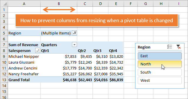
Typically when we make any change or update to a pivot table, the column widths resize automatically to autofit the contents of each cell in the pivot table.

The “update” includes just about every action we take on a pivot table including: adding/removing fields, refreshing, filtering with a drop-down menu or slicer, layout changes, etc.  The autofit feature will resize the column to the width of the widest cell (the cell with the most contents) in each column.

This can be annoying!  Especially when the worksheet contains data in other cells outside the pivot table or any shapes (charts, slicers, shapes, etc.).

Turn Off Autofit Column Widths on Update

Fortunately, there is a quick fix for this.  The pivot table has a setting that allows us to turn this feature on/off.

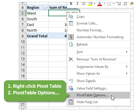
Here are the steps to turn off the Autofit on Column Width on Update setting:

1. Right-click a cell inside the pivot table.
2. Select “Pivot Table Options…” from the menu.
3. On the Layout & Format tab, uncheck the “Autofit on column widths on update” checkbox.
4. Press OK.

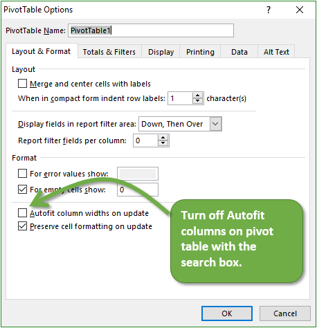
The columns will NOT automatically resize when changes are made to the pivot table.

I also shared this tip in my post on how to create a search box for a slicer.

Shortcut to Autofit the Column Widths Manually

After turning this feature off, there may be times when you want to resize the columns after modifying the pivot table.  We can do this pretty quickly with a few keyboard shortcuts.

Make sure a cell is selected inside the pivot table, then press the following.

1. Ctrl+A to select the pivot table body range.
2. Alt,h,o,i to Autofit Column Widths.

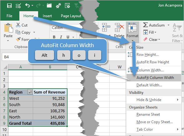
That keyboard shortcut combination will resize the columns for the cell contents of the pivot table only.

If you want to include cell contents outside of the pivot table, then press Ctrl+Space after Ctrl+A.  Ctrl+Space is the keyboard shortcut to select the entire column.

Change the Default Pivot Table Settings

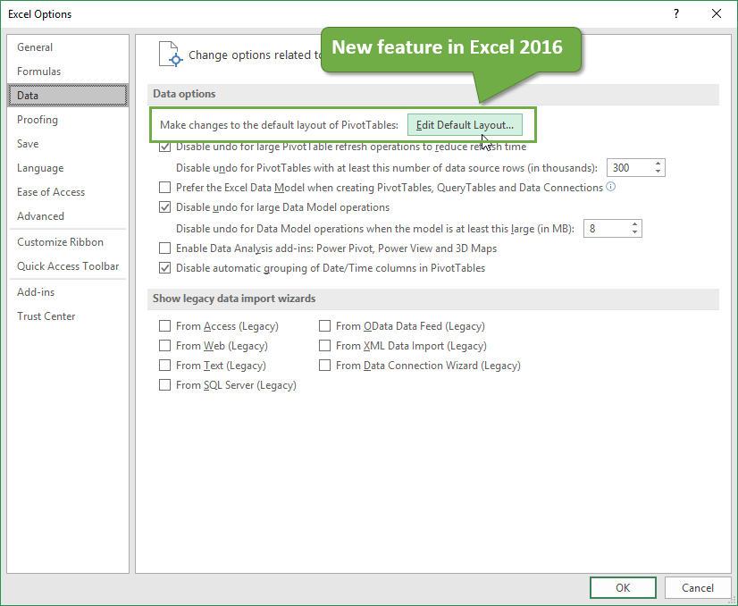
In the latest version of Excel 2016 we can now change the default settings for most pivot table options.  This means we can disable the Autofit column width on update setting on all new pivot tables we create.  This will save us time from having to manually change this setting each time we create a pivot table in the future.

Here are the steps to change the default pivot table settings.  This applies to Excel 2016 (Office 365) only.

1. Go to File > Options.
2. Select the Data menu on the left sidebar.
3. Click the Edit Default Layout button.
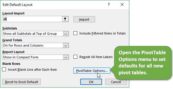
4. Click the PivotTable Options… button.
5. Uncheck the Autofit column width on update setting.
6. Press OK 3 times to save & close the Excel Options menu.

The default settings will apply to all NEW pivot tables you create.  I will do a follow-up post that explains this new default settings feature in more detail.  Again, it's only available on the latest version of Excel 2016 (Office 365 Current Channel).

If you are on an Office 365 ProPlus subscription, then you might be on the Deferred Channel, which might not have this update yet.  Here is an article on how to switch the Current Channel.

Macro to Turn Off Autofit Columns on All Pivot Tables

If your workbook already has a lot of pivot tables, and you want to turn Autofit off on all pivot tables, then we can use a macro for this.

Here is a VBA macro that turns off the Autofit column width setting on all pivot tables in the workbook. The macro loops through all the worksheets in the workbook, and all the pivot tables on each worksheet to turn off the setting. You can also use this to turn the setting back on, by changing the HasAutoFormat property to True.

Sub Autofit_Column_Width_All_Pivots()
'Turn off Autofit column widths on update setting
'on all pivot tables in the active workbook.

Dim ws As Worksheet
Dim pt As PivotTable

  'Loop through each sheet in the activeworkbook
  For Each ws In ActiveWorkbook.Worksheets
  
    'Loop through each pivot table in the worksheet
    For Each pt In ws.PivotTables
    
      'Autofit on column widths on update setting
      'change to True to turn on
      pt.HasAutoFormat = False
    
    Next pt
  Next ws

End Sub

The macro can be copied and pasted to a code module in your Personal Macro Workbook and used on any open workbook. Checkout my free video series on the Personal Macro Workbook to learn more.

Also, checkout my article on the For Next Loop for a detailed explanation on how these types of loops work in VBA.

Note, the macros will work on all versions of Excel.

Macro to List Autofit Column Setting for All Pivot Table

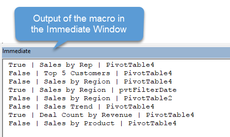
Here is a macro that will list the current value of the Autofit column width setting for all pivot tables in the workbook. The Debug.Print line outputs the results to the Immediate Window in the VB Editor.

Sub List_Pivot_Autofit_Setting()
'Create a list of the current Autofit column width
'setting for each pivot table in the active workbook.
'List is printed to the Immediate Window (Ctrl+G)

Dim ws As Worksheet
Dim pt As PivotTable

    For Each ws In ActiveWorkbook.Worksheets
        For Each pt In ws.PivotTables
            Debug.Print pt.HasAutoFormat & " | " & ws.Name & " | " & pt.Name  
        Next pt
    Next ws

End Sub

The output structure is:

HasAutoFormat value | Worksheet Name | Pivot Table Name

The HasAutoFormat value will be True if the setting is on, and False if the setting is off.

Additional Resources on Pivot Tables & Macros

• How Do Pivot Tables Work?
• Introduction to Pivot Tables and Dashboards [Video 1 of 3]
• How to Add a Search Box to a Slicer to Quickly Filter Pivot Tables and Charts + Video
• 5 Ways to Use the VBA Immediate Window in Excel
• The For Next and For Each Loops Explained for VBA & Excel
• Free Video Series on Getting Started with Macros & VBA

I hope that helps save some time and frustration with the pivot table columns resizing.  Please leave a comment below with any questions or other tips you have for this issue.  Thank you! 🙂