How to Add a Search Box to a Slicer to Quickly Filter Pivot Tables and Charts + Video

Bottom line: Learn how to add a search box to a slicer to quickly filter your pivot tables, pivot charts, or Excel Tables.  Includes a video tutorial that explains the setup in detail.

Skill level: Intermediate

Video Tutorial: How to Add a Search Box to a Slicer

Download the File

Download the file to follow along.

Problem: It's Hard to Navigate Slicers with Lots of Items!

Kati asked a great question about adding a search box to a slicer.  She has a slicer with over 200 items (names) in it, and it takes a lot of time to scroll horizontally through the slicer to find a name.

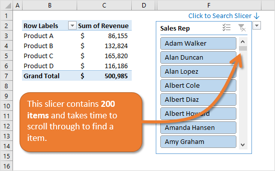
How Can We Add a Search Box to the Slicer?

Unfortunately there is no built-in way to add a search box to a slicer in Excel.  So this solution is a bit of a workaround.

The good news is that it does NOT require any macros or coding.  This solution uses the filter drop-down menu in another connected pivot table, and it is pretty easy to implement.

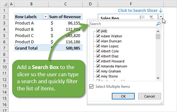
Note: The filter search box was introduced in Excel 2010 for Windows, so this solution will work in the 2010, 2013, or 2016 versions for Windows.  The solution will also work for the Mac 2016 version of Excel.

Step-by-Step Instructions

The video above explains how to add the search box to the slicer.  Here are the basic steps that I explain in the video.

1. Insert a slicer on the worksheet.
2. Make a copy of the pivot table and paste it next to the existing pivot table.
3. The new pivot table will also be connected to the slicer.  The slicer is connected to both pivot tables.
4. Remove all fields from the areas of the new pivot table.
5. Add the slicer field to the Filters area of the new pivot table.
6. Move the slicer on top of the cell that contains the filter drop-down button in the Filters area of the new pivot table.
7. Adjust the column width so the filter button is just to the right of the slicer.
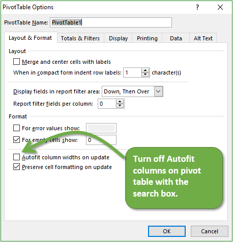
8. Turn off the Autofit column widths option on the new pivot table. (Right-click pivot table > PivotTable Options…)
9. Hide the column that contains the field name in the Filters area of the new pivot table.

Now you should be able to click the filter drop-down button and use the Search box to quickly find items in the field (slicer) and apply filters.

Keyboard Shortcuts

In the video I mention that you can press the letter “e” on the keyboard to place the text cursor in the search box.

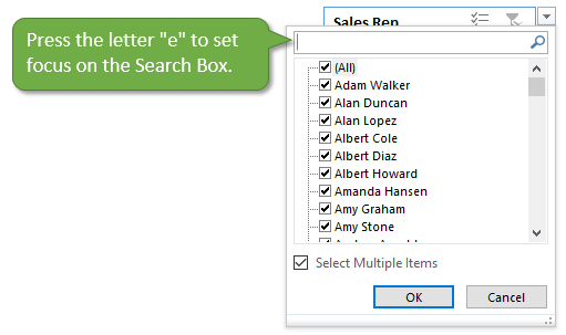
Checkout my article on 7 Keyboard Shortcuts for the Filter Drop Down Menus for more shortcuts for this menu.

You can also add a Hyperlink to the cell that contains the Filter Button.  Then press Alt+Down Arrow to open the menu and jump the cursor into the search box.

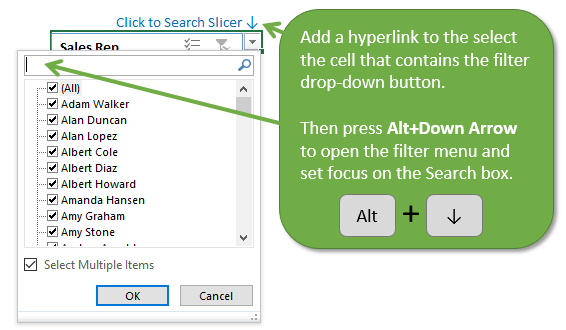
Those shortcuts will make it really fast to get to the search box to filter the slicer.  The hyperlink text also alerts your users that there is a search box available for the slicer.

Use the Slicer Search Boxes on Multiple Slicers in Dashboards

The slicer search boxes are great for dashboards and pivot charts too.  You can repeat the process to setup search boxes for all the slicers in your dashboard.

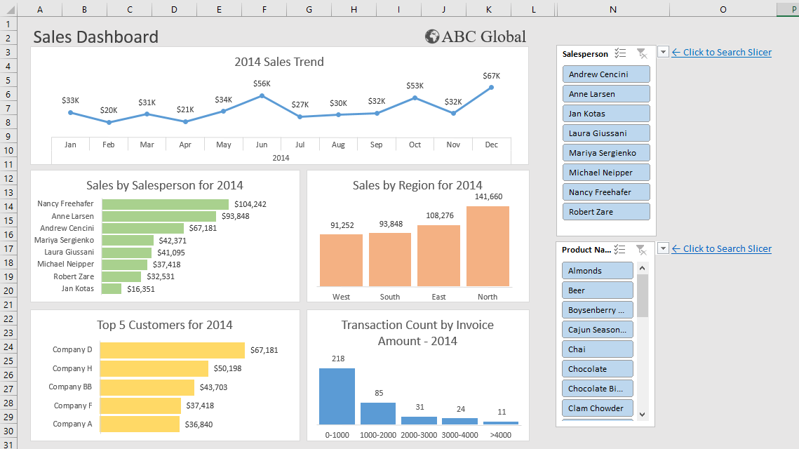
Checkout my free video series on pivot tables and dashboards to learn how to use pivot tables to create the dashboard in the image above.  It's easier than you think! 🙂

I also have an article that explains how to create a list of all the slicers in your workbook.

Alternate Solutions

Wow, there has been a lot of great feedback and questions about this technique!  Here are some alternate solutions to help navigate slicers with a lot of items.

I added a file in the download section above that contains these alternate solutions.

#1 – View the Name of the Filtered Item

Dennis had a great question about not being able to see the item that is selected in the slicer, after you perform the search.  Unfortunately, the slicer will not automatically scroll to the item that is selected in the search.

So you might type a search and apply a filter for a name that is way down in the list.  You won't be able to see that selection anywhere.

One quick workaround is to add the Sales Rep field to the Filters Area of the pivot table.  I recommend this as a best practice anyways because it helps you quickly see what filters are being applied to the pivot.

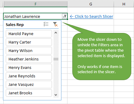
If your slicer is on a dashboard that filters multiple pivots or charts, then you can simply move the slicer down one row to make the filter field visible.  That cell in the pivot table will display the name of the item that is being filtered.

#2 – What if Multiple Items are Applied to the Filter?

The technique above works great if there is only one item selected in the filter/slicer.  If there are multiple items then you will see (Multiple Items) in the Filters cell.

That doesn't help us very much!

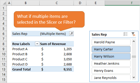
There are a few ways to list out all items that are applied in the filter.

Rob Collie has an article that explains a simple way using the Rows area of another pivot table.

Another way is to use Power Pivot and the CUBERANKEDMEMBER function.  Rob Collie has another article that explains that in more detail.

You can also use VBA and Jan Karel Piertse has an article with a UDF (macro) to list the selected items.

#3 – Add a Parent Grouping to Filter the Slicer with Another Slicer

Another solution to this problem is to create a shorter slicer (with less items) that can filter down the long slicer.

In this example I added a slicer that contains the 1st Initial of the names in the Sales Rep field.

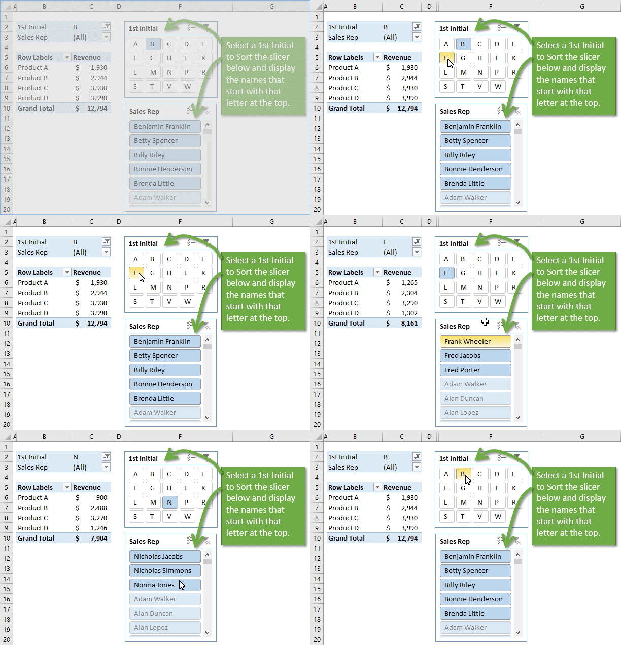
The 1st Initial slicer allows the user to first select the first initial of the name they are looking for.  The Sales Rep slicer will then display a list of the names that start with that initial at the top of the Sales Rep slicer.

This makes it much faster for the user to navigate through the list by narrowing down their selection with the 1st Initial field (slicer).

Checkout this blog post and video for instructions on how to setup the slicer to filter another slicer.

Will You Add Slicer Search Boxes to Your Pivot Tables and Charts?

Please leave a comment below with any questions or suggestions.