Bottom line: Learn how to create month to date (MTD) calculations in your pivot tables for month-over-month, quarter-over-quarter, or year-over-year comparisons.
Skill level: Intermediate
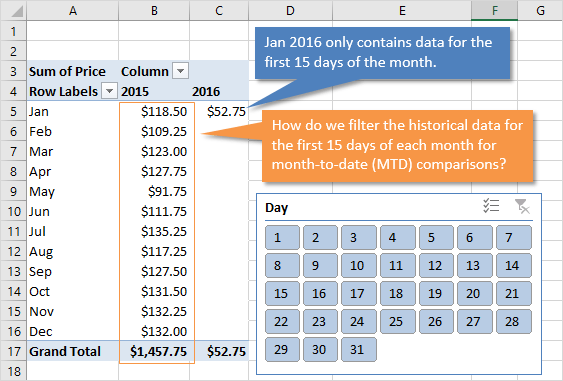
Task: The boss wants to see a report that shows the numbers for the first 15 days of every month (This was actually a great question submitted by Christopher).
Problem: As you can see in the pivot table above, the numbers for Jan 2016 are much lower than Jan 2105. This is because we only have data for the first 15 days of Jan 2016 and 31 days worth of data for Jan 2015.
So we need to find a way to calculate the month to date (MTD) numbers for the other months in the year.
Video Tutorial: How to Filter Pivot Tables for MTD Comparisons
Additional resources:
- Video series on Pivot Tables and Dashboards – includes more on date groupings
- Video on Excel Tables for Beginners
- Guide and video on how to use slicers
Download The Example File
Download the example file to follow along.
The following file contains calculations for the week of the month or year. See the comment below for more info.
Solution: Filter for Days of the Month with a Slicer
The video above explains this entire solution, if you don't like reading. 🙂
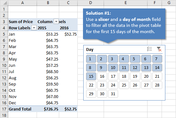
One simple solution is to filter the pivot table to only include transactions that occurred in the first 15 days of every month.
We can apply this filter with a slicer, but first we will need to add a column to our data set for the day of the month.
Note: Slicers are available in Excel for Windows 2010 and beyond, Mac 2016 and beyond. If you have an older version I have an alternate solution below that uses formulas instead of slicers.
Step 1: Add a column that contains the day of the month
Fortunately, Excel has a function called DAY that makes this really easy.
The DAY function will return the day of the month from a date value.
=DAY(serial_number)
The DAY function just has one argument, serial_number. The serial_number is a date value.
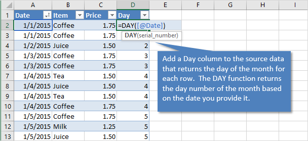
So we can add a column to our source data for the day of the month. We will just enter the DAY formula in cell D2. This formula references the date in the same row in cell A2.
Now just copy the formula down and you will have an entire column filled with the day of the month for each transaction (row).
Step 2: Add a slicer to the pivot table for the new Day field
We can now filter the pivot table for a range of days using a slicer for the Day field.
Important: You will need to refresh the pivot table to see the new field. If you are NOT using an Excel Table for the source data then you will need to change the Data Source Range to include the new column.
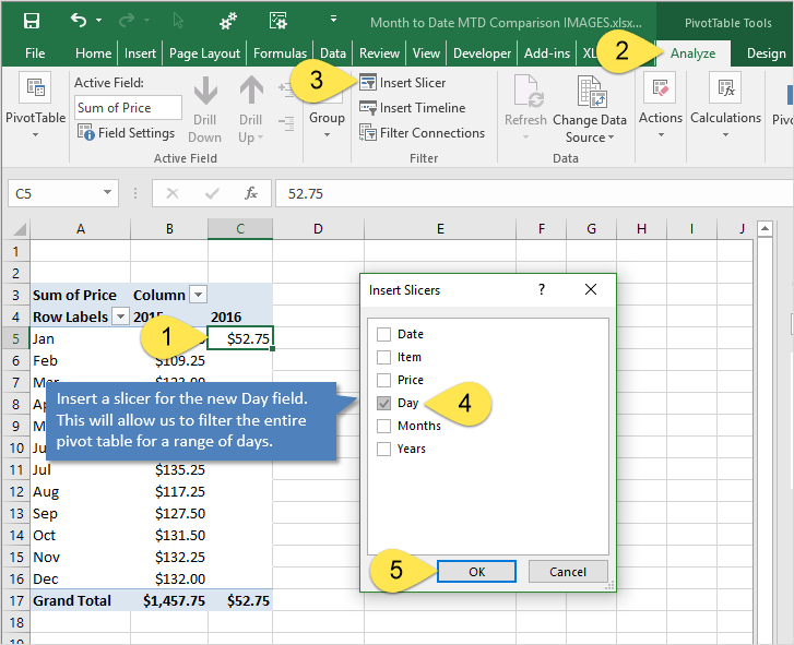
Here are instructions on how to insert a slicer:
- Select any cell inside the pivot table.
- Go to the Analyze/Options tab in the ribbon and press the Insert Slicer button.
- You will see a list of all the fields in the pivot table.
- Click the check box for the Day field.
- Click OK
The slicer will be added to the worksheet next to the pivot table.
You can change the layout to match mine by changing the number of slicer columns to 7, then resize the slicer to view the numbers in the slicer buttons.
Step 3: Filter the pivot table with the slicer for day ranges
We can now filter the pivot table for the first 15 days of the month.
Left-click and hold the “1” button in the slicer and then hover the mouse over the “15”. Release the mouse button and days 1 to 15 will be selected.
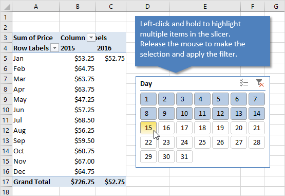
Since the Months are in the Rows area, each cell in the Values area will be filtered for the first 15 days of the month.
This allows us to view the MTD numbers for each month, and also make month over month or year over year comparisons. Awesome!
Alternate Solution: Create a MTD Calculation in the Source Data
The 1st solution requires that your version of Excel has slicers (Excel for Windows 2010 and beyond, Mac 2016 and beyond).
It also requires you to manually select items when new data (days) are added to the source data.
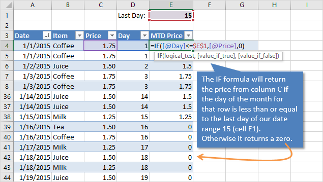
We can also calculate the MTD amount using an IF formula. I added this solution to the example file with more detailed explanation.
The MTD Price field is added to the Values area of the pivot table to give us the same result. The advantage is you don't have to worry about filtering the data for the new days. This is great if you are updating the report with new data every day.
Checkout my article on How to Write an IF Statement Formula for more details on the IF function.
Leave a comment below if you are interested in learning more about how it works, and I will be happy to create a video on it.


Very interesting Jon
what if my day column is setup as 01/10/2015 08:34:11
with the time included, =Day(serial) returns 01/01/1900 00:00
Hi Jim,
Great question! If the value in the cell is a date with a time value then the DAY function should still work.
It looks like you just need to change the formatting of the cell with the DAY formula. You can change it to General or a number format. This will display the day as a number.
I believe the cell is currently set to a date format if it is returning a date like that.
Let me know if that helps.
Thanks!
Excellent!
Can we take this a step further to weeks?
Thank you.
Hi Novzar,
Yes, that is a great question! We could add columns in the source data for Week of Year (1-52) or Week of Month (1-5).
Excel has a function called WEEKNUM that calculates the week of the year. It is a very simple function and you just feed it a date. It also has a second argument that allows you to specify what day the week starts on. By default it starts on Sunday. Put a 2 for the second argument if you want the week to start on Monday.
The WEEKNUM will return the week of the year. There can actually be up to 54 weeks depending on when the first day of the year is.
The formula for the week of month uses the WEEKNUM function but is a little more advanced. It looks like the following.
=WEEKNUM(A2)-WEEKNUM(DATE(YEAR(A2),MONTH(A2),1))+1
Don’t let it scare you though. It is basically taking the week number of the year and subtracting the week number for the first month of the month of the date in cell A2. Let me know if you have more questions about it.
This formula will return the week number of the month. There can actually be up to 6 weeks in the month depending on when the first day of the month is.
Once you have the new columns in the source data, you can then refresh the pivot table and add slicers.
I added another file in the download section above that includes these calculations. Check it out and let me know if you have any questions. Thanks!
How about adding the MTD field for user’s selection?
=IF([@Day]<=$E$1,"MTD","BoM")
so that user may select
"ALL" for full month data;
"MTD" for month to date data:
"BoM" for balance of month data.
Cheers,
Thanks for the suggestion MF! Balance of month could be used for forecasting purposes to see how many sales were done for the remainder of the month historically.
thanks nice informaition
Thanks Ameena!
Hi Jon,
Am thrilled by your tutorials.they are so awsome.
I want to be extemely good at excel.Please lead me through the way.
Looking forward to hearing from you soon.
Regards,
Erick.
Thanks Erick! I am really happy to hear you are enjoying the tutorials.
Great and helpful tutorial! Thanks heaps
Thanks Jen! 🙂
What if i have to Check Year To Date? with a data pool of more than 6 years???
Hi Jon,
I am trying to create M-o-m analysis of Balance Sheet. The data which I am using is ytd balance. Si say if I download data for Feb it would include Jan+Feb month Balance. Similarly for March it will have Jan, Feb and March data.
I am confused over the term MoM when applied to Balance sheet. Can you help me understand does MoM means Feb YTD vs March YTD or Feb MTD vs March MTD .
Regards
Jatin
Thanks
Hello Jon,
Firstly, thank you for sharing your knowledge on Excel.
I’m unable to get my head around this WEEKNUM Solution. So I shall be breaking it down so that you can point out where my understanding is wrong.
Let’s consider a cell say “A84” which is 3rd FEB 2015.
1) WEEKNUM(A84) will give a result as 6, which is 6th Week of the year 2015.
2) WEEKNUM(DATE(YEAR(A84), MONTH(A84),1),2) will give a result as 5, which is 5th Week of the year which is Monday as we have put 2 and also starting tarting of the Feb month
3) Now Subtracting 1)-2) and adding +1 will give a result 2, which is 2nd
Week /*This is part I don’t understand*/
Also if 1st Feb is Monday (considered as starting of the week) then how can 3rd Feb fall in the 2nd week of the month ??