Bottom line: Learn how to group text or number fields to create a slicer that can sort and filter another slicer. This technique is great for slicers that contain a lot of items and are difficult to navigate.
Skill level: Intermediate
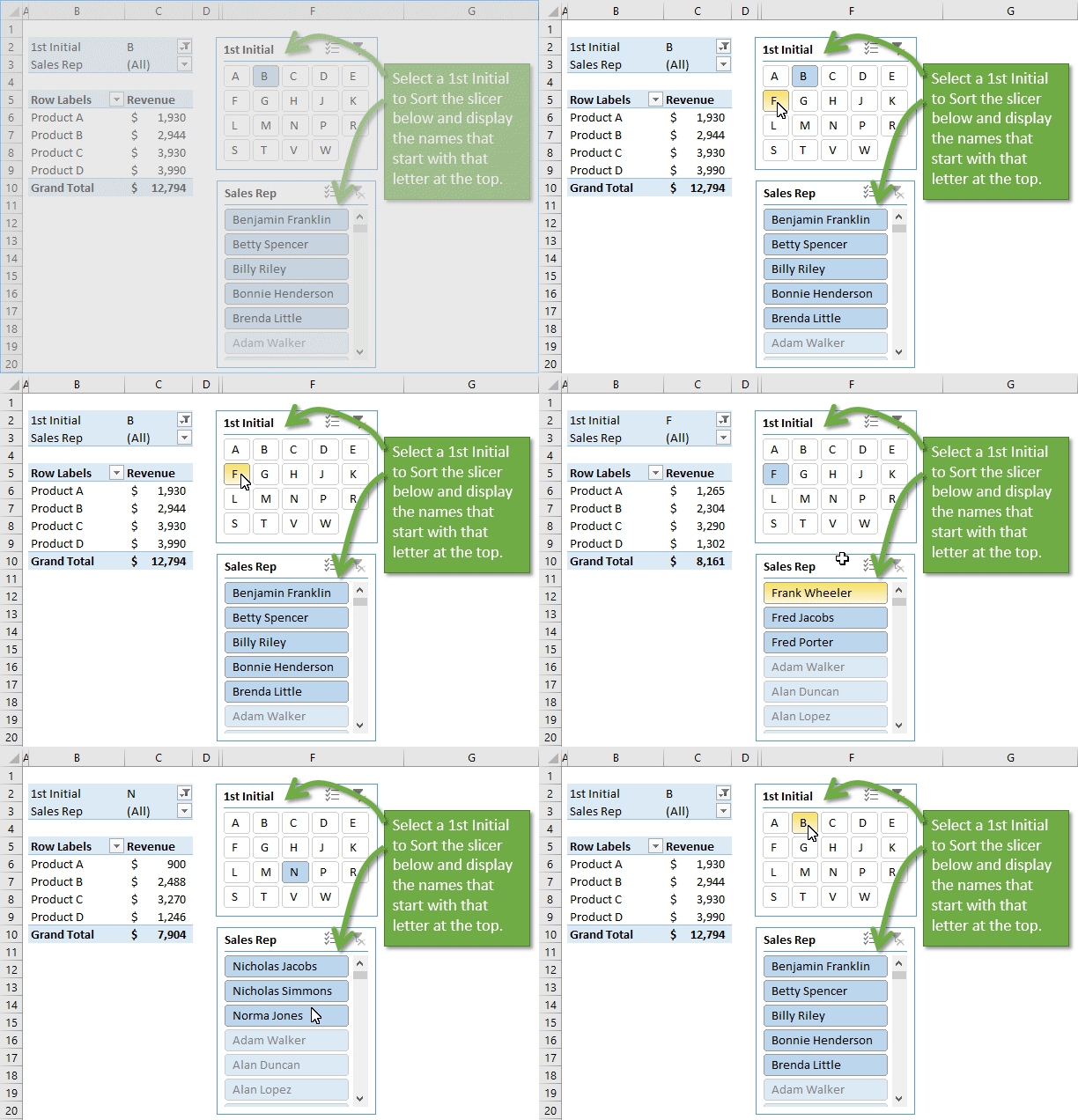
Last week's post about how to add a search box to your slicer raised a lot of great questions on how to tackle a common problem.
The problem is that a slicer can be difficult to navigate through when it contains a lot of items. The user has to scroll horizontally through a long list to find the item they are looking for.
I added some alternate solutions to that post that answer questions about how to view the selected items in the filter/slicer.
Video: Create a Slicer that Sorts Another Slicer
Watch video on YouTube (and hit the Like button!)
Download the File
Download the file to follow along.
How Does This Solution Work?
We are going to create a shorter slicer (with less items) that can filter down the long slicer.
In this example we have a long list of names in our Sales Rep slicer. There are almost 200 items in that slicer.
The “1st Initial” slicer allows the user to first select the first initial of the name they are looking for. The Sales Rep slicer will then be sorted to display a list of the names that start with that initial at the top of the slicer.
This makes it much faster for the user to navigate through the list by narrowing down their selection with the 1st Initial field (slicer).
Add a Parent Grouping Field to the Source Data
This technique is actually pretty easy to setup. We first need to add a field to the source data that contains the first initial for each Sales Rep.
This can easily be accomplished with the LEFT function. The left function returns a specified number of characters from a string or cell value, starting from the beginning of the text/number.
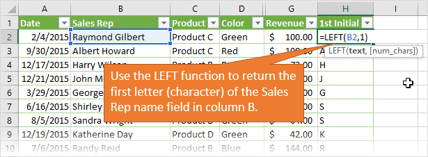
If the Sales Rep name is in cell B2, then the following formula will return the first letter of the text in that cell.
=LEFT(B2, 1)
Copy the formula down the entire column of the data set and you now have a pivot table field for the first initial of each name.
This basically creates a parent level grouping for the Sales Rep names. You can filter the 1st Initial column in your source data for “C” to see a list of all the data for all the reps that have a name starting with “C”.
Add a Slicer for the Parent Level Group Field
Now we just add a slicer to the pivot table for this new field (1st Initial).
It's also best to disable the “Show items with no data last” slicer setting for the parent grouping slicer (1st Initial). This will keep the letters in alphabetical order when an item is selected in either slicer. You can get to the Slicer Settings menu by right-clicking the slicer and selecting Slicer Settings…
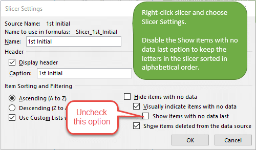
The Show items with no data option also sorts the second slicer (Sales Rep). So you want to make sure this option is enabled for the child slicer (Sales Rep). When an item is selected in the parent slicer, the related child items will be moved to the top of the slicer, and the items with no data will be listed below.
Create Parent Groupings for Text or Numbers
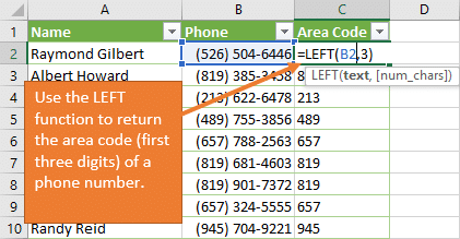
This solution also works for numbers. In the example below I am using the same technique to create parent groups of area codes for phone numbers.
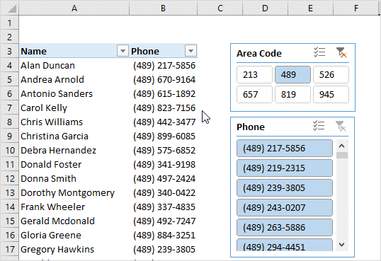
The LEFT function is used to return the first 3 characters from the phone number to create an area code field.
This same technique could be used for all kinds of account codes or id numbers.
I explained a similar technique with dates and days of the month in a recent post on how to do month-to-date (MTD) comparisons with pivot tables.
How Will You Use This Technique?
It would be great to learn how you will use this technique to quickly filter and sort your slicers. Please leave a comment below with questions or suggestions. Thanks! 🙂


Excellent simple solution.
thanks Jon
Thanks Trang!
Thanks for the such a clear and nice tutorials. I learned something new.
Awesome! Happy to hear you learned something. Thanks Prasad!
Excellent solution Jon.
Thanks Muhammad!
What would be the formula if you wanted to do the first letter of the last name? Many thanks for your help Jon
Hi Jim,
Here is a simple formula that will find the first space in the cell’s value, and return the entire string after the first space.
=MID(A1,FIND(" ",A1)+1,LEN(A1))This will work for simple cases where you don’t have middle initials or multiple first names. I hope that helps.
Jon,
Thanks for your help.
Hi. This will work great on my pivot tables. Thanks. One question though, how can this be applied to Business Analytics since I do not have access to the actual data? Thanks.
The question I was trying to answer was about tying the slicers to the pivot tables to make the parent/child relationship work. I downloaded your sample and saw the slicers tied to two pivot tables, which makes perfect sense when it is presented. I’m not sure what PivotTable4 does in your example. I took out the PivotTable4 report connections and the solution still worked fine. An addition to this video might be at the end to click and show the report connections and mention that you can add other pivot tables to the slicers. Once I saw both slicers connected to the pivot table, it made sense, but when trying to design it myself I wasn’t sure if both slicers needed to be connected to the same pivot table to get the parent groupings to function. Thank you for doing all this work to make the video available to us that don’t use slicers every day.
You’re such a blessing to me, Jon! 🙂
This doesn’t work for me. I followed the steps, my slicer settings match yours for both slicers, but the second one doesn’t update based on what I choose in the first.
Hi there, Seasons Greeting, Excel Query : How do I restrict user suppose as shown above If I have a slicer with Main Group as Alpha from Customer, the other slicer will be parent group my query is how can I make a relation, example if I select “A” in First Slicer, the user should not be allowed to the Customer Name starting with “B” if it does so than excel should worn and reset -initialise the previous filters back to original based on the last selection? If there is already a solution than kindly guide me / Thanks in advance