Bottom line: Learn a few keyboard shortcuts to select all the cells in a column of the used range. This is a solution for when the Ctrl+Shift+Down Arrow or Ctrl+Shift+End shortcuts don't work.
Skill level: Intermediate
Built-in Keyboard Shortcuts Don't Always Work
Often times we want to select a single column within a range of data. If the column contains blanks, then making the selection with a single keyboard shortcut can be challenging.
Ctrl+Shift+Down Arrow doesn't work because that will select all cells to the last row in the worksheet because all cells below the active cell are blank.
Ctrl+Shift+End doesn't work because all cells to the end of the used range (cell E14) will be selected. We then have to hold Shift and left arrow a few times to only select the single column.
So, I have two techniques that can help with problem.
Method #1: Excel Tables and Ctrl+Space
The first solution is to use Excel Tables. When our data is in an Excel Table, we can use the keyboard shortcut Ctrl+Space to select the column of the active cell in the Table.
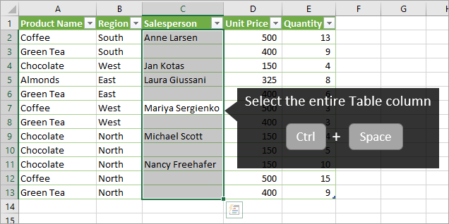
Ctrl+Space will only select the data body range of the column, meaning the header row is excluded.
With the entire column selected we can copy/paste data, apply conditional formatting, delete the contents, or take any other action on all the cells in the column.
It's also good to know that pressing Ctrl+Space a 2nd time will select the entire Table column including the Header. Pressing Ctrl+Space a 3rd time will select the entire worksheet column.
Checkout my video on a Beginner's Guide to Excel Tables to learn more about this awesome feature of Excel. If you have used Tables, but don't like the weird formulas, you can turn those off.
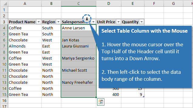
Select a Table Column with the Mouse
If you are more of a mouse user, there is also a shortcut to select the Table column with the mouse:
- Hover the cursor over the top-half of the header cell until it turns into a down arrow.
- Then left-click to select the data body range of the column.
- Left-click again to include the header cell in the selection.
It can be challenging to get the cursor in the correct spot for it to turn into a down arrow. The mouse cursor has to be in the top half of the header cell. It's pretty precise, and takes a little practice.
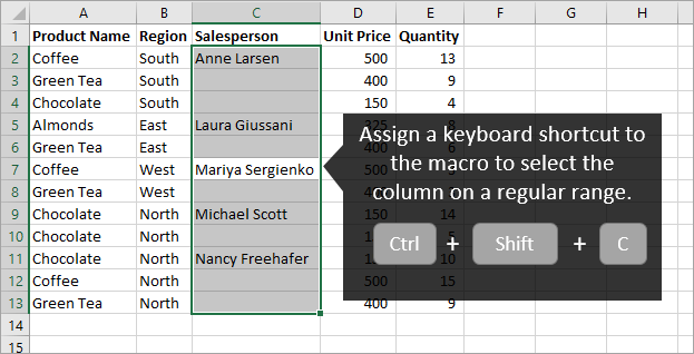
Method #2: Select the Column with a Macro
Even if you are an avid Table user and fan, there's a good chance that your data is not always going to be in a Table. So we need a backup plan…
We can use a macro to mimic the behavior of how Ctrl+Space works in a Table. We can then assign a keyboard shortcut to the macro.
This macro uses the CurrentRegion property of the active cell (the cell the user has selected). The current region is defined as a range bounded by any combination of blank rows and blank columns. This usually returns the used range of data that the activecell is inside of.
This means that if we have multiple ranges of data on the same sheet, we should be able to use the macro to select the entire column of the range of data that the active cell is currently in.
Here is the macro. You can copy and paste it to a code module in your Personal Macro Workbook. Then assign a keyboard shortcut to the macro. Please see the video above for details on how to assign a keyboard shortcut to a macro.
Sub Select_Column_With_Blanks()
'Select all cells for the column of the activecell
'in the current region of data (used cells)


Dim lFirstRow As Long
Dim lLastRow As Long
Dim rActive As Range

    'Store reference of active cell to activate after selection
    Set rActive = ActiveCell

    'Exit if current region is a single cell
    If ActiveCell.CurrentRegion.Count = 1 Then Exit Sub

    'Find the last used cell in the columns of the current region
    'Attempts to account for blank rows in the data by using Range.Find
    'to find the last used cell in the column of the current region.
    On Error Resume Next
        lLastRow = ActiveCell.CurrentRegion.EntireColumn.Find( _
                    What:="*", _
                    After:=ActiveCell.CurrentRegion.EntireColumn.Cells(1, 1), _
                    LookAt:=xlPart, _
                    LookIn:=xlFormulas, _
                    SearchOrder:=xlByRows, _
                    SearchDirection:=xlPrevious, _
                    MatchCase:=False).Row
    On Error GoTo 0

    'Find the first used row in the current region
    lFirstRow = ActiveCell.CurrentRegion.Row

    'Exit if any errors in setting the rows
    If lFirstRow = 0 Or lLastRow = 0 Then Exit Sub

    'If the region contains a header row (bold font cells) then offset start by 1 row
    If Intersect(ActiveCell.CurrentRegion, ActiveCell.EntireColumn).Cells(1, 1).Font.Bold = True Then
        lFirstRow = lFirstRow + 1
    End If

    'Select the range within the column
    Range(Cells(lFirstRow, ActiveCell.Column), Cells(lLastRow, ActiveCell.Column)).Select

    'Activate the orginal active cell
    If Not Intersect(rActive, Selection) Is Nothing Then
        rActive.Activate
    End If

End Sub
The macro should work most of the time. However, if there are blank cells surrounding the active cell, then the current region might be a smaller range than the data range you are trying to select. It's not always easy to figure this out with code, but CurrentRegion gets us close.
The macro uses the Range.Find method to find the last used cell in the columns of the current region. Checkout my article and video series on 3 ways to find the last used cell in a sheet with VBA for more details on this method.
If the macro doesn't work for you in a certain situation, leave a comment below with a link to a screenshot. We might be able to continue to modify and improve the macro for more data layouts.
Other Methods?
What other methods do you use to select a column in a data range? Please leave a comment below with any suggestions or questions. Thanks! 🙂


Jon,
OMG works like a dream, thank you! Quick question: in my VB window, in my Personal.xlsb list, I’m adding more macros but they’re all listed as “Module 1, Module 2….”), but I saw in your demo that yours actually have names reflecting the macro purpose. If I choose one of the modules, I can see in the right window the name (top right), but it’d nice to see that name instead of “Module #” in the list…is this stupid easy to do? 🙂
Thanks for your great tutorials!
Hi Peter,
in case you have not yet found it – this is in the properties of the module, there you can set the name.
Cheers
Ralph
Hmm, I do this with and without tables sometimes, but I’ll
– freeze the header row,
– use the ctrl+down on the column next to the one that has blank cells,
– move the active cell over to that column after I’ve reached the bottom,
– shift+click header title & shift+down.
Now the column w/ blank cells is selected. Hope that made sense. I use this method all the time…b/c I always forget about ctrl+space. =p
Thanks for the suggestion Carrie! I forgot to mention that there is a shortcut for selecting the Table column with the mouse. I added a section to the article above with instructions. Here is a screenshot.
It’s a good one to know if your data is in a Table, and you don’t remember Ctrl+Space. 🙂
Well in tables I generally right click a column and go to “Select”. But that’s a neat trick too, thanks. =)
Another great tip! Thanks again for sharing. 🙂
Thanks for sharing. Works great for me.
Awesome solution – thanks Carrie!
Jon,
Thanks for providing this code. Selecting a range or column with lots of blanks has always been a pain. The code you posted prompted me to think of another option.
For me, most of the time, the data starts in row 2. As such, the code below seems to work consistently and effectively but I’m very interested in getting your feedback. Based on the active cell, it selects the range from the cell in row 2 down to the last non-blank row. Do you see any issues with this?
Sub Select_Column()
Dim ColNum As Long
Dim lRow As Long
ColNum = ActiveCell.Column
lRow = Cells(Rows.Count, ColNum).End(xlUp).Row
Range(Cells(2, ColNum), Cells(lRow, ColNum)).Select
End Sub
Hi Jeff,
Thanks for posting the code. This will work as long as the last cell in the used range or current region contains a value.
The macro might produce unexpected results if there are blank cells at the end of the column of the active cell. Here is a screenshot with an example.
When I run the macro on a cell in column C, the macro is uses the Range.End or Cells.End method to find the last used cell in the column of the active cell ONLY. In this case we might want to expand that search for the last cell to the other columns in the sheet.
We can do this with the Range.Find method. The solution I posted above uses the Range.Find method to look through all columns of the CurrentRegion, and find the last used cell in those columns. In the case of this example, Range.Find would find Row 13 as the last used Row.
I have an article and video series that explains both Range.End and Range.Find in more detail.
3 Ways to find the last used cell on a sheet with VBA
Range.Find has more parameters, and looks scary at first, but it is a very powerful method to learn. There are many use cases for it.
Here is your macro, modified with the Range.Find method.
Sub Select_Column_Range_Find()

Dim ColNum As Long
Dim lRow As Long

ColNum = ActiveCell.Column

lRow = Cells.Find(What:="*", _
                    After:=Range("A1"), _
                    LookAt:=xlPart, _
                    LookIn:=xlFormulas, _
                    SearchOrder:=xlByRows, _
                    SearchDirection:=xlPrevious, _
                    MatchCase:=False).Row

Range(Cells(2, ColNum), Cells(lRow, ColNum)).Select

End Sub
In this case it will look in all the cells in the sheet, and find the last used cell anywhere on the sheet.
In my solution above, I modified this to only have Range.Find look in the columns of the CurrentRegion. So, if there is another table of data in other columns on the sheet, it will not account for those columns in the search for the last used cell.
That solution doesn’t work if you have multiple tables listed in the same column down the page.
It’s challenging to come up with a perfect solution that will work every time here…
Please let me know if you have any questions. Thanks again and have a nice weekend! 🙂
Hello Jon,
Thanks for giving valuable excel tutorial for us. I learned basic excel through your blog and video tutorial. Again thanks for giving information regarding excel by email.
I have one question for you.
How can I earn in five figure (in Lacs) with MS Excel?
Waiting for your Reply
Hi Jon
Thanks for your great emails.
I wonder if you would be willing to help me?
I need to delete Rows from a spreadsheet imported from another source, the problem is that each report has different rows that need deleting each time. Sometimes it’s rows 1-6 and then 50 to 55 and then other times it’s rows 1 to 10 and perhaps 60 to 67 – sometimes more below that.
I am not experienced with VBA – I did watch your Webinar which was great.
But this is beyond me.
I would be most grateful if you could help.
Thanks a lot.
Useful shortcut.
Something has changed in Excel. All of a sudden, CTRL+Shift+Down selects all the way down to the last record, even though I have a few blank cells in between. Any idea what could have changed?
I’m trying to modify your code to work on rows, but it fails. See Below:
Sub Select_Row_With_Blanks()
‘Select all cells for the column of the activecell
‘in the current region of data (used cells)
Dim lFirstColumn As Long
Dim lLastColumn As Long
Dim rActive As Range
‘Store reference of active cell to activate after selection
Set rActive = ActiveCell
‘Exit if current region is a single cell
If ActiveCell.CurrentRegion.Count = 1 Then Exit Sub
‘Find the last used cell in the columns of the current region
‘Attempts to account for blank rows in the data by using Range.Find
‘to find the last used cell in the column of the current region.
On Error Resume Next
lLastColumn = ActiveCell.CurrentRegion.EntireRow.Find( _
What:=”*”, _
After:=ActiveCell.CurrentRegion.EntireRow.Cells(1, 1), _
LookAt:=xlPart, _
LookIn:=xlFormulas, _
SearchOrder:=xlByColumns, _
SearchDirection:=xlPrevious, _
MatchCase:=False).Column
On Error GoTo 0
‘Find the first used row in the current region
lFirstColumn = ActiveCell.CurrentRegion.Column
‘Exit if any errors in setting the rows
If lFirstColumn = 0 Or lLastColumn = 0 Then Exit Sub
‘If the region contains a header row (bold font cells) then offset start by 1 row
If Intersect(ActiveCell.CurrentRegion, ActiveCell.EntireColumn).Cells(1, 1).Font.Bold = True Then
lFirstColumn = lFirstColumn + 1
End If
‘Select the range within the row
Range(Cells(lFirstColumn, ActiveCell.Rown), Cells(lLastColumn, ActiveCell.Row)).Select
‘Activate the orginal active cell
If Not Intersect(rActive, Selection) Is Nothing Then
rActive.Activate
End If
End Sub
You switched the row and column order in the Cells function. This code works for me:
Sub Select_Row_With_Blanks()
‘Select all cells for the column of the activecell
‘in the current region of data (used cells)
Dim lFirstColumn As Long
Dim lLastColumn As Long
Dim rActive As Range
‘Store reference of active cell to activate after selection
Set rActive = ActiveCell
‘Exit if current region is a single cell
If ActiveCell.CurrentRegion.Count = 1 Then Exit Sub
‘Find the last used cell in the columns of the current region
‘Attempts to account for blank rows in the data by using Range.Find
‘to find the last used cell in the column of the current region.
On Error Resume Next
lLastColumn = ActiveCell.CurrentRegion.EntireRow.Find( _
What:=” * ”, _
After:=ActiveCell.CurrentRegion.EntireRow.Cells(1, 1), _
LookAt:=xlPart, _
LookIn:=xlFormulas, _
SearchOrder:=xlByColumns, _
SearchDirection:=xlPrevious, _
MatchCase:=False).Column
On Error GoTo 0
‘Find the first used row in the current region
lFirstColumn = ActiveCell.CurrentRegion.Column
‘Exit if any errors in setting the rows
If lFirstColumn = 0 Or lLastColumn = 0 Then Exit Sub
‘If the region contains a header row (bold font cells) then offset start by 1 row
If Intersect(ActiveCell.CurrentRegion, ActiveCell.EntireRow).Cells(1, 1).Font.Bold = True Then
lFirstColumn = lFirstColumn + 1
End If
‘Select the range within the row
Range(Cells(ActiveCell.Row, lFirstColumn), Cells(ActiveCell.Row, lLastColumn)).Select
‘Activate the orginal active cell
If Not Intersect(rActive, Selection) Is Nothing Then
rActive.Activate
End If
End Sub
Thank you, thank you, thank you! I knew there was a better way then just mindlessly holding ctrl-shift-down arrow, or going to the bottom, pressing Shift, going back to the top… Today I took the two minutes needed to find your blog post, and now my new best friend is ctrl-space.
Another great thing about this shortcut is it works on filtered columns, so after I’ve started a COUNTIF and realize that the table column I’m counting in is filtered, it doesn’t matter. I used to have to cancel the formula, go to the other table, unfilter, go back to the first table and start over.
TAB or SHIFT-TAB changes the pointer position within a selected range. From there you can use the arrow keys to adjust. You have to experiment to get the hang of it. Not as intuitive as 1-2-3.
Thank you for this helpful tip. On the macro how can I change it to select all cells from my cursor is located and below. This macro select the whole column.