5 Reasons to Use an Excel Table as the Source of a Pivot Table

Bottom line: Learn why using an Excel Table as the source of a pivot table can save time and prevent errors.

Skill level: Beginner

Do You Love Excel Tables?

Excel Tables are one of those hidden gems of Excel.  They are an extremely useful feature that can save us a lot of time when working with lists or sets of data.

Tables are becoming more popular, but a lot of people still don't use them.  I believe this is mainly due to the “weird” formulas that are used in Tables.

The formulas are called structured references, and they can be turned off if you don't want to use them.  Structured reference formulas are actually very useful once you understand how they work, but that is a whole other topic.

Checkout my video on a Beginner's Guide to Excel Tables if you are not using this feature yet.

In this post I want to focus on why you should use Tables for the source data range of your pivot tables.  So let's get into it.

 #1 – Adding New Data & Preventing Embarrassment

Have you ever added new data to the bottom of your source data, and then forgot to update the pivot table(s) to include the new rows of data?

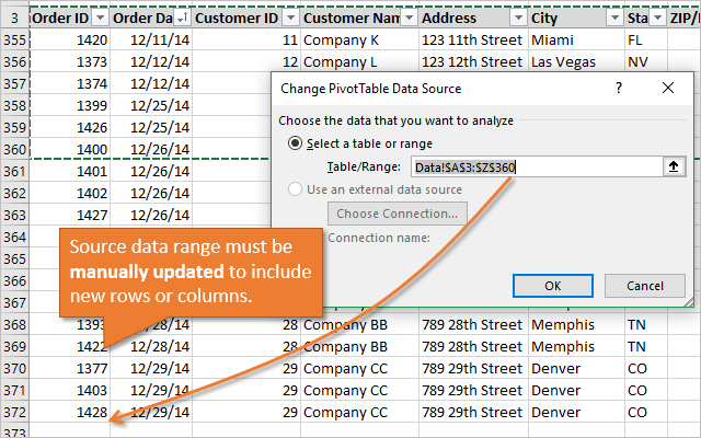
The better question is, how many times has this happened to you?  I'll admit that this has happened more than once in my career, and it's an embarrassing mistake.

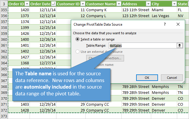
Using Excel Table as the source data range of the pivot table prevents this mistake.  When we paste data below a Table, the Table automatically extends to include the new data.  Since the pivot table(s) reference the Table name as source data range, instead of a range reference, the new data is automatically included in the pivot table.

The only step you have to remember is to refresh the pivot table(s).

For me, this one reason alone is enough to always use Tables as the source data range.

#2 – Eliminate Maintenance on Multiple Pivot Tables

Typically we create multiple pivot table reports on one source data range.  If we use a regular range for the source, we have to update every single pivot table when we add new data (rows or columns) to the source.  This can be very time consuming if your workbook has dozens of pivot tables.  There is always a chance we miss one, and again suffer from that embarrassing mistake…

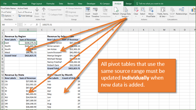
When we use a Table as the source range, we do NOT need to change the source data range when we add new rows or columns to the end of the table.

All pivot tables that use the Table as the source data range will be refreshed because they share the same pivot cache.  This means you can just refresh one pivot table, and all the others that use the same Table as the source will also be updated.  Here is an article that explains more about the pivot cache and how pivot tables are connected.

#3 – Prevent Errors When Creating Pivot Tables

Pivot tables are picky, and require the source data to be in the right format and layout.  I have a source data checklist that explains more about the 8 steps to formatting your source data.

One of those steps is deleting blank columns.  We cannot create a pivot table from a source data range that contains blank columns.  Excel gives us the following error message.

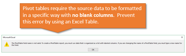
The PivotTable field name is not valid.  To create a PivotTable report, you must use data that is organized in a list with labeled columns.  If you are changing the name of a PivotTable field, you must type a new name for the field.

This error message causes a lot of confusion.  It should say, “Your data cannot contain blank columns or a header row that contains blank cells.  Each column must have a descriptive name in the first (header) row of the source data range.”

The advantage of using an Excel Table is that it does NOT allow us to have blank cells in the header (top) row.  All cells in the header row must contain a value.  If they don't, a value will be inserted in the cell.  The value will be “Column” with a number after it: Column1, Column2, etc.

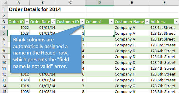
Even if your source data has blank columns, those columns will get a header name when you insert the Table.  This means you will not get that error message when creating a pivot table.

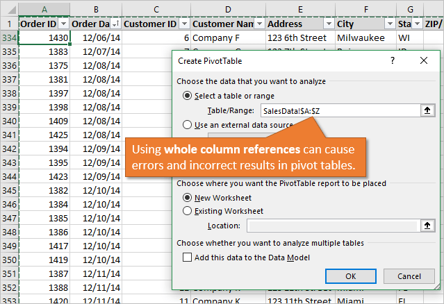
#4 – Avoid Whole Column References

Another “trick” I see used a lot to avoid maintenance is to use whole column references for the source data range.  We can just reference the entire columns of the source data range in the pivot table, so we don't have to change the last row number when new data is added.

In theory this would help eliminate the issues I explained in #1 and #2 above.  However, whole column references come with their own set of potential issues.

Here's a quick list of reasons to not use whole column references:

• If any data is accidentally added to the bottom of the sheet below the actual data range, it will also be included in the pivot table.  This can lead to bloated pivot tables, incorrect results, and issues with the grouping feature not working due to blank cells in a column.
• You cannot add formulas below the actual data range to help tie out numbers.
• Whole column references do not include new columns added to the right of the data range.  This still requires maintenance to update the source ranges.

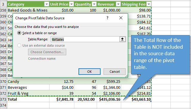
If we use an Excel Table instead we don't have to worry about these issues.  We can add formulas below the data range, and we can also use the Totals Row feature of the Table to summarize columns.   The Totals Row is NOT included in the pivot table.

#5 – Prevent the Filter Controls Error with Connected Slicers

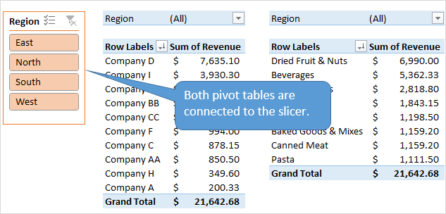
If you've seen my video series on pivot tables and dashboards, then you know we can connect a slicer to multiple pivot tables and pivot charts to create interactive dashboards.  This is a very powerful feature of Excel.

However, if we use a regular range as the source of our pivot tables, we first have to disconnect the slicers before changing the source data range.  We then have to reconnect all the slicers after the update.  This can be very time consuming, and is a tedious manual process.

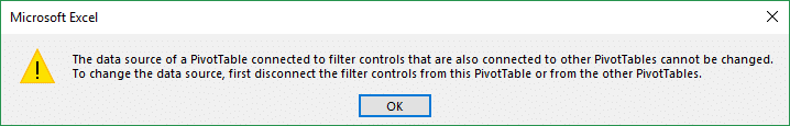
I have an article on how pivot tables and slicers are connected, that explains this issue in more detail.  The ultimate solution is to use a Table as the source range.  This prevents the error and we do not have to disconnect the slicers to add new data to the source.

How to Use Tables with Pivot Tables

Now that we know why to use Tables, you might be wondering how to set it up.

Creating a New Pivot Table from a Table

Here are instructions to create a new pivot table from a Table:

1. Select any cell in the Table.
2. Go to the Insert Tab on the Ribbon and click the “Pivot Table” button.  There is also a “Summarize with Pivot Table” button on the Table Design tab that does the same thing.
3. The Create PivotTable window will open and the Table name should automatically be referenced in the Table/Range box.
4. Choose where you want the pivot table to be placed, new or existing worksheet.
5. Click OK.

The new pivot table will be created using the Table as the source data range.

Changing the Data Source for an Existing Pivot Table

If you have an existing pivot table that uses a regular range as the source, you can change it to use a Table as the source.  Here's an animated screencast with the instructions below:

1. Go to the source data range and Insert a Table (Insert tab on the Ribbon > Table).
2. Go to the existing pivot table and select a cell inside the pivot table.
3. Go to the Options/Analyze tab on the Ribbon and click the “Change Data Source” button.
4. The Change PivotTable Source Data window will open.
5. Select a cell inside the Table.
6. Press Ctrl+A.  This shortcut will select all cells in the Table and automatically insert the Table Name in the Table/Range box.
7. Click OK.

The pivot table will now use the Table as the source data range, and benefit from all the reasons mentioned in this article.

Other Reasons To Use Tables with Pivot Tables?

Well, there are 5 good reasons to start using Tables with Pivot Tables.  Checkout my video on a beginner's guide to Tables for more reasons to use this awesome feature of Excel.

Tables are also used with tools like Power Query and Power Pivot, so it's good to get experience with how Tables work.

Do you have any other reasons to use Tables with pivot tables.  Please leave a comment below with suggestions or questions.  Thank you! 🙂

Free Training Webinar on Pivot Tables

Next week I'm hosting a free webinar on “The 5 Secrets to Understanding Pivot Tables”.

During the free webinar I am going to explain how we can use pivot tables to quickly summarize our data for interactive reports and dashboards.

I am going to share my screen and jump into Excel to explain how pivot tables work, and some of the most critical steps for using this powerful tool.  This is one of those Excel skills that will help you save time with your job, and impress the boss. 🙂

Click here to register for the webinar

Spots are limited so get registered today.  It's free!