How to Prevent #SPILL Errors in Excel Tables  

Bottom Line: Learn a couple of ways to prevent errors when using dynamic array formulas that produce spill ranges in Excel Tables.

Skill Level: Intermediate

Watch the Tutorial

Download the Excel Files

You can follow along with the tutorial using the files below. I've included both the Before and After Excel files.

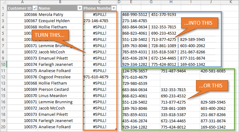
Why You Might See a #SPILL Error in Your Excel Table

#SPILL errors occur when there essentially isn't enough space for Dynamic Array Functions to spill their results. (For an explanation of these functions and how they work, see this post: Dynamic Array Formulas & Spill Ranges.)

For example, below I'm using a FILTER function in an Excel Table, and it is returning #SPILL errors in column C. That's because the formula is designed to look up a customer ID on another sheet and return the phone number associated with it. The problem comes in when there is more than one phone number. The spill range is larger than the single cell that the Excel Table allows for that formula value.

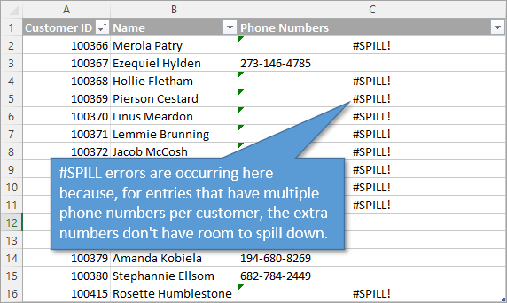
If this function were written outside of an Excel Table, the spill range would expand and show the multiple results. But because this is in an Excel Table, the formula gets copied down to the cells below. This essentially blocks the spill results.

You can see that some entries don't have a #SPILL error. That is because there is only one phone number associated with that particular customer.

Workarounds for the #SPILL Error

There are a couple of different ways to take care of this problem.

1. Combine the Values Using TEXTJOIN

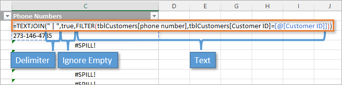
We can wrap our existing FILTER function with the TEXTJOIN function. This will combine the multiple results into one cell, separated by a delimiter (a character or mark of our choice).

The first argument to identify for the TEXTJOIN function is the Delimiter. You can use a comma, a space, a slash, a pipe, or whatever you think would work best. Enclose your delimiter in quotation marks when you are typing out this portion of the formula. Also, be sure to include one or more spaces before/after the delimiter depending on how separated you want your results to be from one another.

I find that with lots of numbers like these, the comma doesn't quite separate the entries visually as well as something like space, the pipe symbol, and another space: " | "

The next argument is Ignore Empty, which means the formula will skip over entries that have nothing in them. Set that argument to true by just typing the word true.

The last argument is Text, and that is the array that the FILTER function is returning. In other words, the FILTER formula that already exists becomes the final argument for the TEXTJOIN function.

All together, our formula looks like this:

With our formula complete, the text is combined together (yet separated with delimiters) for any entry that has more than one result.

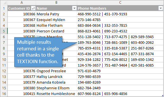
One of the drawbacks of this solution is that because multiple results are combined into a single cell, it makes it difficult to analyze or further work with the individual entries. You might want to use formulas or pivot tables to take a closer look at some of the results, but that can be challenging if they are all combined together.

That leads us to our next solution.

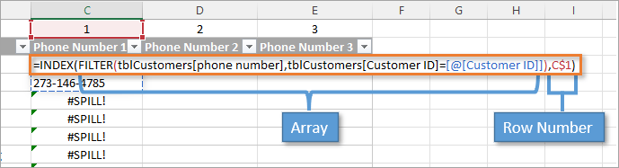
2. Split Values into Their Own Cells Using INDEX

Just as with the previous solution, we are going to keep the FILTER formula as an argument in our new INDEX function. In this case, it will be the first argument for INDEX, which is Array.

The second argument is Row Number. This is the row number that we want to return from the filter's spill range. You can type the number 1 to indicate the first row of your spreadsheet, but I prefer to make it a little more dynamic. Instead of typing 1, I can select a cell that is in Row 1 and then add a dollar symbol ($) in front of the row number reference (but do not add a dollar symbol in front of the column letter reference). Example: C$1

This makes my row reference absolute and my column reference relative so that the values calculate correctly when copied in cells to the right.

You do not need to identify any other arguments for this formula, so the final result looks like this.

Hit Enter. The formula will copy down, and each of the cells in the column will show the first phone number for each customer. As you copy the formula in columns to the right, the second and third phone numbers will appear, if applicable.

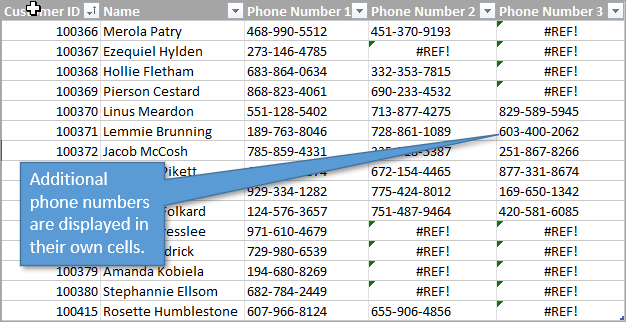
Removing the #REF! Errors

If you don't like seeing those #REF! errors, you can wrap your entire formula in the IFERROR function, adding quotation marks with nothing in between them to indicate you want nothing to appear in those cells.

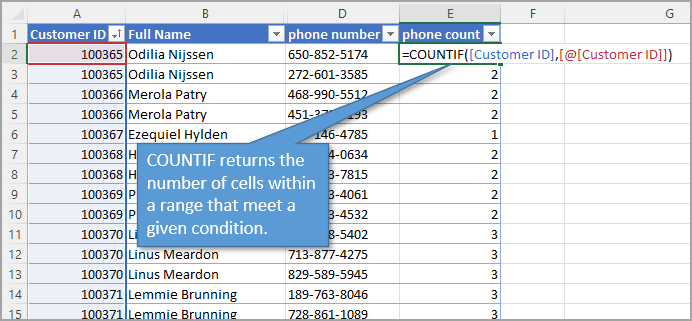
How many columns do I need?

A small drawback to this solution is that you have to figure out how many extra columns to add to your table. A relatively easy way to do this is to go to your source data and add a column where you can enter a COUNTIF function. The COUNTIF function will tally any duplicate Customer IDs and return the number of times that ID occurs in the data.

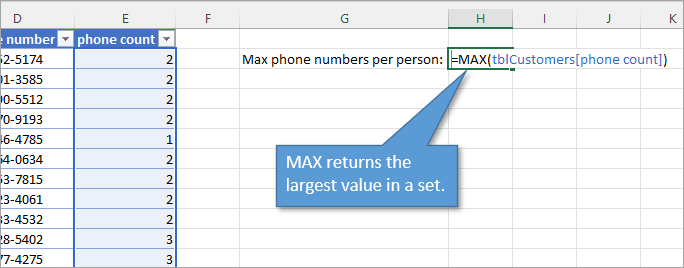
From there, if your data set is relatively small, you can glance down the list to see the highest number. That would be the number of columns you need for your table. If your data set is large, you can use the MAX function to quickly tell you what the highest value is.

Related Posts

Take a look at these tutorials on related topics:

• Return Multiple Values for a Lookup Formula in Excel with FILTER and UNIQUE
• 3 Ways to Combine Text in Excel – Formulas, Functions & Power Query
• Excel Tables Tutorial Video – Beginners Guide for Windows & Mac

Conclusion

These solutions will work for any Dynamic Array formula that returns a spill error. It's not specific to the FILTER function.

I hope they are helpful to you. If you have any other comments, tips, or questions in regards to spill ranges, I'd love to hear them in the comments below.

Until next time!