Distinct Count Report with Dynamic Array Formulas

Bottom Line: Learn how to use the UNIQUE and COUNTIF functions to count unique rows based on multiple columns of data.

Skill Level: Intermediate

Video Tutorial

Download the Excel File

You can download the example file from the video here. I've included both the original file and the file with the solution:

Solving the Data Analysis Challenge

This post and video are the third in a series featuring solutions to a challenge I posed to readers. The inspiration for this data analysis challenge came from Rob, one of our Elevate Excel Training members.

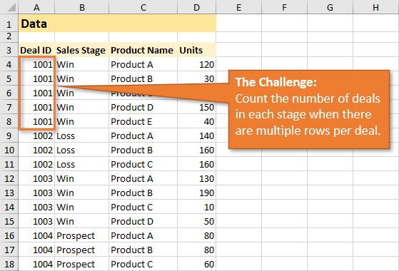
The challenge is to create a summary report of deal count by sales stage. The issue is that there are multiple rows for each deal (transaction) in the source data. So we need to find a way to just count the unique rows for each deal.

To see the first set of solutions to the challenge, using Excel Tables and Power Pivot, watch this tutorial: 2 Ways to Calculate Distinct Count with Pivot Tables. The second solution solved the same challenge using Power Query: How to Count Unique Rows with Power Query.

Today we will use dynamic array functions to solve the challenge. Unfortunately, this option is only available on the latest version of Excel with a Microsoft 365 subscription, so if you are running an older version, you'll have to stick with the solutions listed above. Checkout my post & video on Dynamic Array Formulas for more info on the compatibility.

Dynamic Array Functions to Return a Unique Count

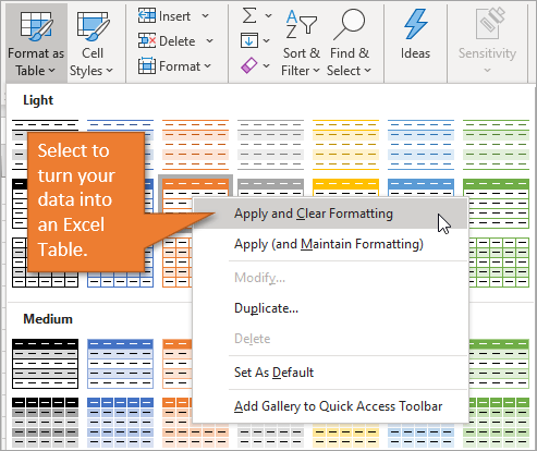
Our first step is to convert our data into an Excel Table. To do that, just select any cell in the data set, and click on Format as Table on the Home tab. Right-click on the table format you want and select Apply and Clear Formatting.

Hit OK when the Format as Table window appears.

The next steps involve using dynamic array formulas to create spill ranges of output data. If you're new to Dynamic Array Formulas & Spill Ranges, click the link to learn more about them. We will be using the UNIQUE and COUNTIF functions for this particular solution.

The UNIQUE Function

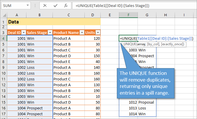
This function analyzes a set of data looking for unique entries, and then it returns those values in a spill range. It has three basic arguments but we only need to specify the first argument, which is array.

For our report, we want to specify the array as both the Deal ID and Sales Stage columns, so we just hover over the headers for both of those rows and select them.

The formula would be: =UNIQUE(Table1[Deal ID]:[Sales Stage])

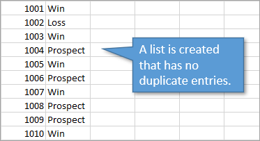
Once you've identified the array, just hit Enter. You'll have a new range of unique values from the two columns.

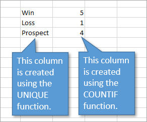
The next step to create our report is to use the UNIQUE function again, this time to create a list of sales stages. So our array for this one is just the Sales Stage column and our formula would read:

=UNIQUE(Table1[Sales Stage])

Our next step will be to count all of the deals that are in each stage. For that we will use a different dynamic array function:

The COUNTIF Function

The COUNTIF function tallies up the number of entries that meet a certain criteria. In our case, we want to count the number of deals found in each sales stage. To write this function, type =COUNTIF, then identify the range. The entire spill range that we just created with the UNIQUE function can serve as our range for COUNTIF. To indicate this spill range, just type the range's home cell (the top-left cell in the range) followed by the # symbol. In my example, the range is F4#.

(Quick note: The data that we are actually counting is found in the second column of the spill range, but because we know there is no danger of finding duplicate data in the first column, we are safe to reference the whole spill range. If your spill range were to have columns with matching data, you would want to only reference the column you need instead of the whole range.)

The second argument in the COUNTIF function is criteria, and that will be the list of unique sales stages that we created above. To reference that spill range, we use I4#.

So the complete formula would look like this:

=COUNTIF(F4#,I4#)

And that basically creates the report we're looking for: the number of deals found in each sales stage.

Pros and Cons

The biggest advantage of using the Dynamic Array Functions lies in the fact that the report we've made is completely dynamic. Any changes made to the source data are automatically reflected in our report. Unlike the Power Query or Pivot Table solutions, we do not have to refresh any tables to see updated results.

A disadvantage to using the Dynamic Array Functions is that this solution doesn't automatically create a Total row for our report. This is easily remedied, of course, and I have another tutorial which shows you how to do that: Total Rows for Dynamic Array Formulas & Spill Ranges. You'll also need to create headers to format your outcome data like a report.

Another disadvantage of this method is that you lose the ability to filter down further by other columns, such as Product. For that type of flexibility, the pivot table method mentioned earlier is better.

Conclusion

I hope you've learned something new through this series. It's great to learn different ways of solving a problem to keep your mind flexible and to approach things from fresh perspective—both in Excel and in life.

If you have any questions about this particular solution, please leave a comment! See you next time.