Bottom line: Create a summary report that counts transactions by a category when the data contains multiple rows per transaction.
Skill level: Intermediate
Video Explanation
Download the Excel File
You can download the Excel file that contains the source data for the challenge below.
The Challenge
This data analysis challenge is based on a great question from Rob, a member of our Elevate Excel Training Program.
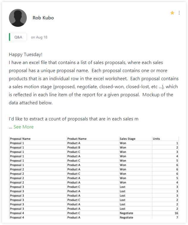
He has sales pipeline (CRM) data and wants to create a summary report of deal count by sales stage. The problem is that each deal/transaction has multiple rows in the source data. The data includes rows for each product in the deal.
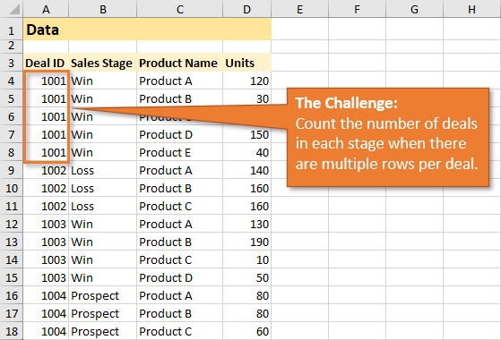
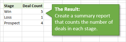
However, Rob only wants to count each deal one time in his summary report by sales stage. Here is an image of what the end result should look like.
Your mission, should you choose to accept it, is to use any of the tools or features in Excel to create the summary report.
Bonus Challenges
I have two additional challenges for you. These are not required, but do force us to think about making the report flexible and dynamic for future updates.
1. Account for New Data
Is it easy to include the new data in your results?
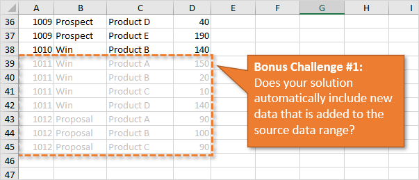
Your solution should be able to easily recalculate the results when new data is added to the source range. I put some additional data on the New Data tab in the workbook. You can copy/paste this below the original source data to test your solution.
We don't want to have to completely recreate the report every time the data is updated.
2. Account for New Sales Stages
What if the stage names change, or new stages are added to the system?
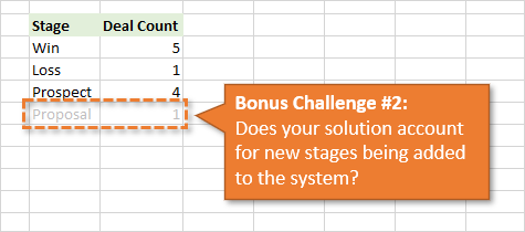
Currently, there are three stages (Win, Loss, Prospect). The data on the New Data sheet includes a new stage, Proposal. Your solution should also be able to automatically include this new stage in the results. Or include it without too much additional work.
Solutions
2 Ways to Calculate Distinct Count with Pivot Tables
How to Count Unique Rows with Power Query
Distinct Count Report with Dynamic Array Formulas
Share Your Solution
I love this question from Rob because there are A LOT of different ways to solve this problem in Excel. And of course, pros & cons to each.
However, I want you to give it a try! Don't worry about it being the “perfect” solution. That probably doesn't exist anyways…
You can leave a comment below or on the YouTube video with a brief description of the tools & techniques you used to solve the challenge. You can also upload your file to any cloud service like OneDrive, Google Drive, or Dropbox and post the share link in your comment.
I will follow-up with a video(s) explaining the most popular techniques and the pros & cons of each. We look forward to seeing your solutions and learning from everyone that participates. Thanks! 🙂


Hi, same as Andrew
format data as a table
insert Pivot table with Add this data to data model
rows – sales Stage
sum – deal ID – change Value Settings to Distinct Count
with this amount of new data the quickest way would be to copy and paste at the end of the table I guess – then refresh pivot…
to make it fully automatically we may use power query, load both tables and append them
Hello John, thank you for this cool challenge. I hope i am the first one with this solution.
1) Make a table out of the data, i named it tbl_data
2) Enter this Formula in B2.B30 in tab “Results”. Enter it as an Array formula IFERROR(INDEX(tbl_data[Deal ID],SMALL(IF(MATCH(tbl_data[Deal ID],tbl_data[Deal ID],0)=ROW(INDIRECT(“1:”&ROWS(tbl_data[Deal ID]))),MATCH(tbl_data[Deal ID],tbl_data[Deal ID],0),””),ROW(INDIRECT(“1:”&ROWS(tbl_data[Deal ID]))))),””)
3) Enter this formula in C2:C30 in tab “Results”: IFERROR(VLOOKUP(B2,tbl_data[[Deal ID]:[Sales Stage]],2,FALSE),””)
4) Enter this Formula in E2:E30 in tab “Results”: IFERROR(INDEX($C$2:$C$30,SMALL(IF(MATCH($C$2:$C$30,$C$2:$C$30,0)=ROW(INDIRECT(“1:”&ROWS($C$2:$C$30))),MATCH($C$2:$C$30,$C$2:$C$30,0),””),ROW(INDIRECT(“1:”&ROWS($C$2:$C$30))))),””)
5) Enter this formula in F2:F30 in tab “Results”: IF(E2=””,””,COUNTIF($C$2:$C$30,E2))
The formula updates automatically in every case mentioned.
Quick if Argument + ifCount –
1 – Cell E4, insert formula =IF(A4=A3,0,B4) and copy down
2 – Cell I4 (under Deal Count heading) insert formula =COUNTIF(E:E,H4) and copy down.
Bonus 1
Create table. Adding new lines auto increase table size and results.
Bonus 2
Add new line with new stage name at bottom of Results and copy Deal Count formula from row above.
This was an excellent challenge. I hope I did it well.
Hello Jon and Rob,
Thank you for the challenge, and I hope you both are doing well.
The challenge for me was deciding what route to take for the end result, so I decided to do a pivotable.
I copied and pasted the data to the results sheet, created a table, and named it tblResults. Then, I inserted a pivot table for the count on the same sheet as tblResults; I added “Stage” in the row and Deal ID in the sum. Once I completed that portion, I went to the new data worksheet and copied and pasted and my table expanded, but I had to redo the the items in the pivot table, like a refresh. I added them back and the new items were counted as well.
Is there another way I can share the spreadsheet. I have not become comfortable with the other tools yet.
I would be more that happy to email it to one of you. Because I would like your feedback.
Thanks,
Great challenge, thanks a lot!
The by far the fastest and easiest is to me the pure and simple Power Query “remove duplicates/group by” solution many others came up with.
However, I tried a formula solution as well:
1. Convert data to table (here named “Data”)
2. Create list of stage per deal (here in sheet Data F4):
=XLOOKUP(
UNIQUE( Data[Deal ID] ),
Data[Deal ID],
Data[Sales Stage]
)
3. In sheet Result A4, get the stage categories:
=UNIQUE( Data[Sales Stage] )
4. In sheet Result B4, count the corresponding values from the list created in step 2:
=COUNTIFS( Data!F4#, Results!A4# )
I tried to skip step 2 to by replacing the first argument in step 4 with the XLOOKUP formula from step 2, both directly and more readable by using LET(). But that just gave me a spilled range of #VALUE errors. I can’t really figure out why, seems counter-intuitive to me. Or?
Hi,
I made the data range into a table to ensure it would be dynamic and then on the ‘Results’ tab I used the UNIQUE function to identify all the current and future stages (‘Win’, ‘Loss’ & ‘Prospect’) rather than hard coding them in, using the following =UNIQUE(Table1[Sales Stage]). This means they will update when a new stage is added.
Then I used the following combination to identify the counts for each stage:
=COUNTA(UNIQUE(FILTER(Table1[Deal ID],Table1[Sales Stage]=A5)))
‘Win’ was obviously in A5. Then I repeated the formula for ‘Loss’ and ‘Prospect’. Once I added in the additional data from the ‘New Data’ tab my summary updated with the new counts and the new ‘Proposal’ stage name.
Hi !
Here’s my take on this challenge (almost the same as Swamy’s from august 27)
1. Convert data range into Excel Table.
2. Name each column as Named Range
(Deal_ID;Stage;Product;Units)
(Makes my formulas easier to read)
FORMULAS
3. In Results sheet cell B5
=UNIQUE(Stage)
4. In Cell C5
=COUNTA(UNIQUE(FILTER(Deal_ID;Stage=B5)))
Copy formula down
With Named Ranges in a Excel Table, new data will be added in Results.
One slight drawback though:
you must remember to copy formula from cell C5 further down
if new Sales Stage is added.
Beyond the challenge, I added a couple of arrays:
Stage Count per Deal & Stage Count per Product.
Link:
https://1drv.ms/x/s!Ag8TOfPLrav0mjXgZRBEpyYrP7G3?e=qJzYbq
no need to copy down formula from C5 if you add “#” after “Stage=B5” to make the formula apply to the whole dynamic array from B5
Hi Jon, I struggled a bit trying to find a solution with the new functions UNIQUE, FILTER and so, but somehow could not get the result trying to get it to work. So, I thought that it should not be that difficult using Pivot table. And it isn’t. So, I created a table of the data and added it to a Pivot table. Row lables is ‘Sales stage’ and values is ‘Deal ID’. ‘Deal ID’ however need to be formatted as Distinct count in the Value field settings. And there you have a pivot table with the distinct values per Sales stage. So, nothing to do with removing duplicates etcetera and grouping by 😉 But for sure there are many ways to get the required result.
Used Excel VBA to copy Stage data to the “Results” spreadsheet, then remove duplicates to get unique Stage names. Put them into an array.
Then copied iD and Stage data to another area of the “Results” spreadsheet and also removed duplicates so I have a unique list of ID and Stage data.
Last, used my Stage array to run “CountIf” against the ID and Stage list
With Data. Added Data
Win. 5 Win 7
Loss 1 Loss 2
Prospect 4 Prospect 4
Proposal 1
No clue as to upload a macro enabled workbook so if you put this VBA code into a module on your test database, you can see how it works.
Option Explicit
Option Base 1
Sub Solutions()
Dim WS1 As Worksheet, WS2 As Worksheet
Dim Arr() As String
Dim DataRow As Integer, NewRow As Integer
Dim LRow1 As Long, LRow2 As Long, LRow3 As Long
Dim SZStage As Integer
Dim SZID As Integer
Dim StageArray() As String, IDArray() As String
Dim i As Long
Set WS1 = Sheets(“Data”)
Set WS2 = Sheets(“Results”)
DataRow = 4
NewRow = 3
LRow1 = WS1.Range(“A:A”).SpecialCells(xlCellTypeLastCell).Row
WS1.Range(“B” & DataRow & “:B” & LRow1).Copy WS2.Range(“H” & DataRow)
WS2.Range(“H” & DataRow & “:H” & LRow1).RemoveDuplicates Columns:=1, Header:=xlNo
WS1.Range(“A” & DataRow & “:B” & LRow1).Copy WS2.Range(“E” & DataRow)
WS2.Range(“E” & DataRow & “:F” & LRow1).RemoveDuplicates Columns:=1, Header:=xlNo
LRow2 = WS2.Range(“H” & DataRow).End(xlDown).Row
SZStage = (LRow2 – DataRow) + 1
LRow3 = WS2.Range(“F” & DataRow).End(xlDown).Row
ReDim StageArray(1 To SZStage)
For i = 1 To SZStage
StageArray(i) = WS2.Cells((DataRow – 1) + i, 8).Value
Next
For i = 1 To SZStage
Range(“I” & (NewRow + i)).Value = WorksheetFunction.CountIf(Range(“F” & DataRow & “:F” & LRow3), StageArray(i))
Next
WS2.Range(“E” & DataRow & “:F” & LRow3).ClearContents
WS2.Range(“H” & NewRow).Value = “Stage”
WS2.Range(“I” & NewRow).Value = “Deal Count”
WS2.Range(“F” & NewRow & “:I” & (NewRow + SZStage)).Font.Bold = True
End Sub
named the columns, created a column where you have to type in the stage name (to allow for new ones) then a countif for the stage name. threw in an if statement for istext so the table doesn’t have a string of zeros
Here is the VBA code I wrote to to the above.
Sub ListUnique() ‘ assume ActiveSheet
Dim A As Variant, v As Variant
Dim C As Collection, K As Collection, R As Range
Dim dataLastRow As Long, outputRow As Long, n As Long
Const dataColumn As Long = 1 ‘ data in column A
Const outputColumn As Long = dataColumn + 1
Const dataFirstRow As Long = 2 ‘ row 1 is header
dataLastRow = Cells(Rows.Count, dataColumn).End(xlUp).Row
Set R = Range(Cells(dataFirstRow, dataColumn), Cells(dataLastRow, dataColumn))
A = R.Value ‘ array of data values
Set C = New Collection ‘ unique items
Set K = New Collection ‘ count of each unique item
On Error Resume Next ‘ ignore error when adding repeated data value
For Each v In A
v = CStr(v)
If v = vbNullString Then v = “BlankCell”
Err.Clear
C.Add Item:=v, Key:=v
If Err = 0 Then
K.Add Item:=1, Key:=v
Else
n = K.Item(v) + 1
K.Remove v
K.Add Item:=n, Key:=v
End If
Next v
On Error GoTo 0
outputRow = Cells(Rows.Count, outputColumn).End(xlUp).Row
Range(Cells(dataFirstRow, outputColumn), Cells(outputRow, outputColumn)).Clear
outputRow = dataFirstRow
For Each v In C ‘ output results
Cells(outputRow, outputColumn) = v & ” = ” & K.Item(v)
outputRow = outputRow + 1
Next v
End Sub
I also figured that the Power Query solution was the easiest to implement quickly AND to easily add more data. I can also make slight changes to the queries I the boss changes his mind and wants to know how many deals by product!!
I also used Power Query but slightly different.
1. Select source data and convert to table
2. Load data to power query from table/range
3. Remove the last 2 columns
4. Select the sales stage column and do a basic group by
5. New column name = Deal Count; Operation = Count Distinct Rows
6. Close and load to existing worksheet as a table
Sub Macro1()
Application.DisplayAlerts = False
On Error Resume Next
Sheets(“1”).Delete
ActiveWorkbook.Sheets.Add
ActiveSheet.Name = “1”
Sheets(“Data”).Select
Range(“A3”).Select
Dim TabRange As Range
Dim TabCache As PivotCache
Dim TabDin As PivotTable
Dim n As Integer
Set TabRange = Cells(3, 1).CurrentRegion
Set TabCache = ActiveWorkbook.PivotCaches _
.Create(SourceType:=xlDatabase, SourceData:=TabRange)
Sheets(“1″).Select
Set TabDin = TabCache.CreatePivotTable _
(TableDestination:=Cells(1, 1), TableName:=”1”)
With ActiveSheet.PivotTables(“1”).PivotFields(“Deal ID”)
.Orientation = xlRowField
.Position = 1
End With
With ActiveSheet.PivotTables(“1”).PivotFields(“Sales Stage”)
.Orientation = xlRowField
.Position = 2
End With
ActiveSheet.PivotTables(“1”).RowAxisLayout xlTabularRow
ActiveSheet.PivotTables(“1”).PivotFields(“Deal ID”).Subtotals = Array(False, _
False, False, False, False, False, False, False, False, False, False, False)
Range(“A12”).Select
With ActiveSheet.PivotTables(“1”)
.ColumnGrand = False
.RowGrand = False
End With
On Error Resume Next
Sheets(“Results”).Delete
On Error Resume Next
Sheets(“2”).Delete
ActiveWorkbook.Sheets.Add
ActiveSheet.Name = “2”
Dim TabDin2 As PivotTable
Set TabDin2 = TabCache.CreatePivotTable _
(TableDestination:=Cells(1, 1), TableName:=”2″)
With ActiveSheet.PivotTables(“Tabela dinâmica1”).CubeFields( _
“[Intervalo].[Sales Stage]”)
.Orientation = xlRowField
.Position = 1
End With
ActiveSheet.PivotTables(“Tabela dinâmica1”).PivotFields( _
“[Intervalo].[Sales Stage].[Sales Stage]”).PivotItems( _
“[Intervalo].[Sales Stage].&[Win]”).Position = 1
ActiveSheet.PivotTables(“Tabela dinâmica1”).CubeFields.GetMeasure _
“[Intervalo].[Deal ID]”, xlCount, “Deal Count”
ActiveSheet.PivotTables(“Tabela dinâmica1”).AddDataField ActiveSheet. _
PivotTables(“Tabela dinâmica1”).CubeFields(“[Measures].[Soma de Deal ID]”), _
“Soma de Deal ID”
ActiveSheet.PivotTables(“Tabela dinâmica1”).CompactLayoutRowHeader = “Stage”
With ActiveSheet.PivotTables(“Tabela dinâmica1”)
.ColumnGrand = False
.RowGrand = False
End With
ActiveSheet.PivotTables(“2”).ChangePivotCache ActiveWorkbook.PivotCaches.Create _
(SourceType:=xlDatabase, SourceData:=ThisWorkbook.Sheets(“1”).UsedRange, Version:=xlPivotTableVersion15)
With ActiveSheet.PivotTables(“2”).PivotFields(“Sales Stage”)
.Orientation = xlRowField
.Position = 1
End With
ActiveSheet.PivotTables(“2”).PivotFields(“Sales Stage”).PivotItems(“Win”). _
Position = 1
ActiveSheet.PivotTables(“2”).AddDataField ActiveSheet.PivotTables(“2”). _
PivotFields(“Deal ID”), “Deal Count”, xlCount
Range(“B6”).Select
With ActiveSheet.PivotTables(“2”)
.ColumnGrand = False
.RowGrand = False
End With
Sheets(“1”).Select
ActiveWindow.SelectedSheets.Visible = False
Sheets(“2”).Select
Sheets(“2”).Name = “Results”
Sheets(“Results”).Select
Sheets(“Results”).Move Before:=Sheets(5)
‘ ActiveWorkbook.Save
Application.DisplayAlerts = True
End Sub
i would like to offer a vba solution for the main problem.
here is the code:
Sub ListUnique() ‘ assume ActiveSheet
Dim A As Variant, v As Variant
Dim C As Collection, K As Collection, R As Range
Dim dataLastRow As Long, outputRow As Long, n As Long
Const dataColumn As Long = 1 ‘ data in column A
Const outputColumn As Long = dataColumn + 1
Const dataFirstRow As Long = 2 ‘ row 1 is header
dataLastRow = Cells(Rows.Count, dataColumn).End(xlUp).Row
Set R = Range(Cells(dataFirstRow, dataColumn), Cells(dataLastRow, dataColumn))
A = R.Value ‘ array of data values
Set C = New Collection ‘ unique items
Set K = New Collection ‘ count of each unique item
On Error Resume Next ‘ ignore error when adding repeated data value
For Each v In A
v = CStr(v)
If v = vbNullString Then v = “BlankCell”
Err.Clear
C.Add Item:=v, Key:=v
If Err = 0 Then
K.Add Item:=1, Key:=v
Else
n = K.Item(v) + 1
K.Remove v
K.Add Item:=n, Key:=v
End If
Next v
On Error GoTo 0
outputRow = Cells(Rows.Count, outputColumn).End(xlUp).Row
Range(Cells(dataFirstRow, outputColumn), Cells(outputRow, outputColumn)).Clear
outputRow = dataFirstRow
For Each v In C ‘ output results
Cells(outputRow, outputColumn) = v & ” = ” & K.Item(v)
outputRow = outputRow + 1
Next v
End Sub
I think Pivot table is best solution to see whatever format he needs.. Sales man wise, product wise, won, lost and prospects wise…
1. Insert table (TblRawData) for existing data – (A6)
2. Clear Stage (H4:H6) values
3. Convert Result Stage (H4) to unique formula – spills below
4. Add Unique Deals area in column P
5. Insert unique TblRawData[Deal ID] in P4 – spills below
6. Look up Sales Stage for each unique Deal ID using Index/Match combined with If to blank rows with no Deal ID value. This formula is copied down 100 rows to accommodate growth in deals
7. Use Countif to count unique deals matching Sales Stage in column H – step 4 above. Test for blank Stage and blank count result
TblRawData grows automatically if new data is pasted in below table range. Unique Sales Stage and Deal ID grow automatically with TblRawData growth. Sales Stage and Deal counts will grow to the limits noted above.
Link to submission –
https://drive.google.com/file/d/1d9DkrNQ-UlAtlA5ktGAi7VNYyT6D_NkE/view?usp=sharing
Forgot to mention – this version works on Excel for Mac. No need for PowerQuery.
My solution
Make data as a table
Use power pivot and add to model this table
Create a power pivot: in the rows use Sales Stage; in the column use Deal Id
Modify the values filed settings of the filed Deal Id applying Distinct Count
by
My solution:
1. Create a column beside the data headed Count and containing the formula: =IFERROR(IF(MATCH(A4,A:A,0)=ROW(),1,0),0). This flags rows with unique Deal IDs.
2. Create a pivot table filter Count = 1, Rows Sales Stage and Values = Count of Deal ID.
I am not familiar with Power Query, finding these sorts of solutions adequate to my needs.
Hi!
PT
1. Make data range into table.
2. Add helper column with name Deal Count and formula: =1/Countif([Deal ID];[@[Deal ID]])
3. Make PT with Sales Stage in row and Sum Deal Count in values
4. Done
Hi fellow Excel lovers.
My first – pretty easy – solution was to use Pivot Table (selecting “Add to Data Model” option on generating the pivot table) with ‘Sales Stages’ in Rows and ‘Distinct Count of DealID’ in Values. Done.
But to make it more challenging I decided to go down the VBA route.
Prerequisites:
1. Source data turned into Excel Table (with the default name “Table1”)
2. Reference to Microsoft Scripting Runtime turned on In VB Editor (Tools -> References -> check Microsoft Scripting Runtime)
High-level overview of the code:
1 | Copies CRM data from the worksheet table into array.
2 | Generates dictionary DealID(key)-SalesStage(value) from this array.
3 | From the first dictionary generates second dictionary SalesStage(key)-Count(value).
4 | Transforms this to array and prints to selected cell in workbook
Link to the Excel file
https://1drv.ms/x/s!AvZS9AXuvdoEyU08I5xgeP94XMlK?e=089gLG
Link to txt file containing the VBA code
https://1drv.ms/t/s!AvZS9AXuvdoEyU_8emMsaEp03zLR?e=OKaZrZ
Daniel
Copy the first two colums to another sheet aplay UNIQUE function and then use COUNT.IF to count the number of wins, loses, etc.
For de second challenge convert the range into Excel tables tte will update automatically if you ad new data o the data is modified.
Hi,
I used this formula to get the variable result
=COUNTIFS(INDEX(UNIQUE(Data!$A:$B),,2),$C3)
where $C3 is ref of “Win”, $C4 = loss , $C5 = Prospect
it is working fine
https://docs.google.com/spreadsheets/d/10UiGaI8tQZipa_tSxO9FhI-G6SBBVaQ77qqLW3zJMSc/export#gid=1154216978
Regards
Deepak
Nice challenge, especially for someone like myself still learning all that Excel can do.
My solution involved using vba, dynamic ranges, VLOOKUP, and data validation. You add new Deal IDs and Sales Stages via user forms, then add data to the Data table on the Data worksheet. I created a worksheet name Calculations that does a lot of the grunt work of summarizing the data, making it possible to sum up the different Sales Stages and ultimately generate the results in the Result table.
My goal was to make it simple enough so that anyone with even the most rudimentary knowledge of Excel could easily add data to the form and update the results, without altering or removing any of the original data entered in the Data table. The link to my file is here:
https://www.dropbox.com/scl/fi/4ujazraxd4xxqiyk1ce2f/Data-Analysis-Challenge-Solution.xlsm?dl=0&rlkey=8prt49ltxap6q0yahpkzs46oj
Someone in the comments used the Advanced Filter to extract the unique records. I had never seen this, so I decided to give it a try. It is awesome, it literally solved the problem in about 5 minutes. Thanks!
I decided to revise my original solution and incorporated the Advanced Filter option. It eliminated the need to create an additional worksheet and a bunch of VBA code to generate a new Dealer ID. I also created some code to automatically update the Result table on the Data sheet whenever column D (Units) was updated. All of the rest of the VBA code I created the first time was able to be transferred to this second solution, with some minor updating. In addition, I kept the data validation list, dynamic ranges, conditional formatting, and the Result table on the Results worksheet from the first solution. The link to the second solution is here:
https://www.dropbox.com/scl/fi/amqf7x30x1dp8hu3w60tn/Data-Analysis-Challenge-Second-Method.xlsm?dl=0&rlkey=5yhm5nksc7bcu8r5liftdwxl5
Solutions to Excel Data Analysis Challenge
Hi,
Since most of the participants demonstrated solutions with either Power Query or Pivot Table, I chose to solve the challenge with a formula.
To be more exact, two formulae: the first using the new dynamic arrays and the second – “traditional”, “old fashioned” functions.
Both solutions are dynamic, either when you add new rows to the original data set or when adding a new category (“Sales Stage”).
Needless to say, both use the Table feature of Excel.
Each solution has two formulae: the first displays the unique categories and the second shows the number of Deal Counts per each Sales Stage.
It should also be stated that each formula can, of course, be dragged downwards as new rows are added to the table, thereby rendering the solutions dynamic.
Now, after the long introduction, let’s get down to business
Solution 1: Using Dynamic Arrays
Formula 1 displays the unique categories (“Win”, “Loss”…..)
Since the name of table I gave the data set is Table1,
The formulae in cells H4:H6 is:
=UNIQUE(Table1[Sales Stage])
Cells I4:I6 show the number of Deal Counts per each Sales Stage:
The formula in these cells is:
=COUNT(UNIQUE(FILTER(Table1[Deal ID],Table1[Sales Stage]=$H4)))
Solution 2: Using “traditional” functions
Formula 1 displays the unique categories (“Win”, “Loss”…..)
Since the name of table I gave the data set is Table2,
The formulae in cells H4:H6 is:
=IFERROR(INDEX(Table2[Sales Stage],MATCH(,COUNTIF(H$3:H3,Table2[Sales Stage]),)),””)
Cells I4:I6 show the number of Deal Counts per each Sales Stage:
=SUMPRODUCT((Table2[Sales Stage]=$H4)/COUNTIFS(Table2[Deal ID],Table2[Deal ID],Table2[Sales Stage],Table2[Sales Stage]))
P.S.
I think that this problem can be solved with Advanced Filter, but I haven’t tried it yet.
Best Regards,
Meni Porat
If you add a # to the $H4 in your count formula in the 1st solution then you only need to enter it once, in cell I4
The formula will spill for as many cells as are needed (no need to fill down)
Yes, jim, I’ve seen Jon’s explanation.
I have Office 365 so I’m not yet completely acquainted with all the intricacies of the new Dynamic Arrays.
BTW, what do you think of my second solution?
Easiest way to do this is Power Query. Create a table with the data set, load it into PQ, group the sales stage and count distinct rows. That’s it. When extra data and new stage names are added, PQ will extract this and automatically load the new values – once you have refreshed the data. Simples and effective! Happy Excelling!
Convert Data to Table–> Unique formula to get stages in sheet –> =COUNT(UNIQUE(FILTER(tblSales[Deal ID],tblSales[Sales Stage]=B4))) to get deal count
Seems very complex in Excel. My solution is pandas:
import pandas as pd
xl = ‘inputs/Data-Analysis-Challenge – 2.xlsx’
df = pd.read_excel(xl, sheet_name=’Data’, skiprows=2, usecols=’A:C’)
grouped_data = df.groupby([‘Sales Stage’]).agg(count=(‘Deal ID’, ‘nunique’))
grouped_data
Use control + T and create a table out of data.
In the cell beside Win enter
=COUNTIF(Table4[Sales Stage],H4). Drag down. When the new
data is added add Proposal to the count list. Drag formula down.
This will give a count of the number of Win, Loss, ect.
I want to identify multiple cells (Eg:which admin expenses) which are linked to particular figure (Eg:Total admin expense) in another work sheet/book. It is difficult to use Trace precedent when 20+ cells are linked from multiple locations. Is there a way to identify multiple cells in another work sheet/book?
5 is not the correct answer for the “Win”, the correct answer must be 6. Codes 1001,1003,1005,1007,1010 and 1011 are having the “Win” stage.
Change Data Set to Table. Define a new Name Deal that is equal to table row Deal ID. I called my table Data, so Deal =Data[Deal ID] is the name definition. Do the same thing for Sales Stage; I called the name Sales.
Enter the following formula in cell I4:
SUM(1/COUNTIF(Deal,Deal)*IF(Sales=H4,1,0))
H4 is the reference for Win. Drag the formula down into I5 and I6. As the table updates, the formula will update. If there are additional Sales Stages added, the formula will work too.
Regarding the last comment, there can be no blank table rows.
Just came across your great question – one year later! Although its been answered very well above I just wanted to chime in with one solution that I have used over the years that has worked really well for me. It took me about 1 minute to get solutions for both questions (the unique/ distinct count as well as the data additions. Here it is:
1. Convert the data into a table (Ctr + T)
2. Add table to Data model (I used power pivot menu)
3. Create pivot table (click PivotTable within power pivot window)
4. Use Distinct Count measure on DealID
5. And lastly, copy ‘new data’ and append to the table and hit refresh. And that’s it.
6. If new categories are needed, just add raw data and repeat step 5 above.
Txs, Charlie
I formatted the data into a table first. Let me know what you think of this:
https://www.dropbox.com/s/5henvrebqc2eug4/Data-Analysis-Challenge.xlsx?dl=0
Well this was a fun problem. No need for tables here. On the Data tab, in cell I4, though it would work in the Results tab too:
{=SUMPRODUCT(–(B$4:INDIRECT(“B”&MAX((A:A””)*(ROW(A:A))))=H4),–(1/COUNTIF(A$4:INDIRECT(“A”&MAX((A:A””)*(ROW(A:A)))),A$4:INDIRECT(“A”&MAX((A:A””)*(ROW(A:A)))))))}
Will do the trick for all criteria. “Prospect” must be entered manually into cell H7, and the formula can be simply dragged for all entries on the left from I4 down. Any additional entries are automatically tabulated by the sumproduct limited to the last column containing actual data. This is an array function, so ctrl+shift+enter.
Convert the data to a table ‘Data’.
Create a new column E named “double”
Place in the new column the formula =E5=E4 which returns “TRUE” or “FALSE”
In I4 place formula COUNTIFS(Data[Sales Stage];H4;Data[Double];FALSE)
I am quite new to using Excel but I enjoyed this question!
To complete this question I started by turning the data into a table (ctrl+T) and defined a name for the “Deal ID” and “Sales Stage” columns (just for ease of use). Next I created a dynamic table using the offset function. I combined this with the unique function to separate each Deal ID =UNIQUE(OFFSET(Deal_ID_and_Sales_Stage,0,0)). After this I created a Win/Loss/Prospect count by using the countif function =COUNTIF((G52#),”Win”) where G52# was the location of my dynamic, unique table.
As I said I am quite new to excel so if there anything I could do more efficiently please let me know!
I just used the formula:
=SUMPRODUCT(–(UNQIUE(A:B)=H4))
Which, for this scenario, worked fine? Not sure if I’ve missed anything by using this? I’d love to know if I’ve missed something!
Great Challenge Jon
I thought it was straight forward. I did a pivot table by stage and deal and then I added the additional data at the end of the data table and I did a refresh all and then to check I did change data source to see it has captured everything and it did. please reply as I want to know if I am doing something wrong