2 Ways to Calculate Distinct Count with Pivot Tables

Bottom Line: Learn two ways to solve the data analysis challenge, calculating distinct count, with pivot tables.

Skill Level: Intermediate

Video Tutorial

Download the Excel File

I've included both the original file and the solution file for you to download here:

Counting Unique Rows

In this post, we're going to take a look at two different ways to do a distinct count using pivot tables. These two methods were submitted as solutions to the data analysis challenge that you can find here:

Excel Data Analysis Challenge

To summarize the challenge, we want to create a summary report of deal count by stage, but there are multiple rows per deal in the CRM data. So we have to find a way to create a distinct count (counting unique rows) for each deal so that we can sum them up.

By the way, thank you to anyone who submitted a solution to the data challenge! There were a lot of great submissions.

Solution #1 – Using a Helper Column

The great thing about this solution is that it can be used in any version of Excel.

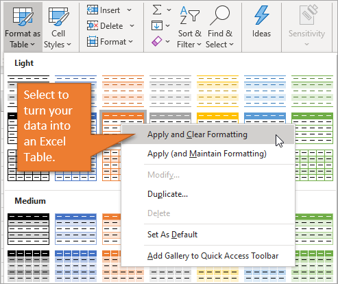
Start by turning your data into an Excel Table. To do that, just select any cell in the data set, and click on Format as Table on the Home tab. Right-click on the table format you want and select Apply and Clear Formatting.

Hit OK when the Format as Table window appears.

Now that your data is in Table format, add a helper column to the right of the table and label it Deal Count. Use the COUNTIF function, with the range being the Deal ID column, and the criteria being the cell in the Deal ID column that corresponds with the row you are in.

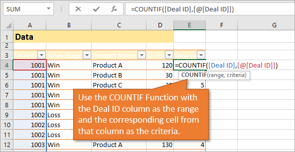
The formula will return the number of rows for each Deal ID number. If we divide the formula into the number 1, we will get fractions in each of those cells that when added together will count one entry for each deal.

The change to the formula can be seen in green here:

=1/COUNTIF([Deal ID],[@[Deal ID]])

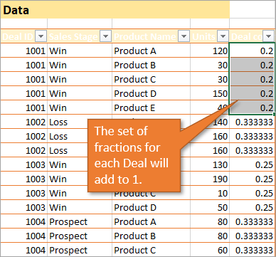
Now that we have these fractions that will give us a distinct count when we create our pivot table, we can go ahead and create the pivot table by choosing Pivot Table on the Insert tab.

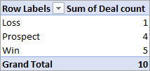
To create our summary report using the new pivot table, put the Sales Stage in the Rows area and Deal Count in the Sum of Values area.

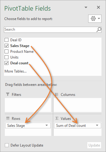
This will give us the summary report we are looking for, with a count of deals in each sale stage.

The nice thing about using a pivot table is that as we add or delete source data entries, we can refresh the pivot table ( Alt + F5 ) to include those changes.

Solution # 2 – Using Power Pivot

This solution is only available for versions of Excel that are 2013 or later for Windows.

We still want our data formatted as an Excel Table, but we don't need a helper column for this solution.

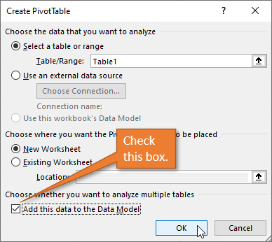
This time, when we create our pivot table, we are going to check the box that says Add this table to the Data Model. (Data Model is another term for PowerPivot.)

When you build your pivot table this time, you are going to drag Deal ID to the Sum of Values area.

That initially gives us numbers we don't want in our summary report. To fix this, we want to right-click on the Sum of Deal ID column header and select Value Field Settings. This will open a window where we can choose Distinct Count as a calculation type.

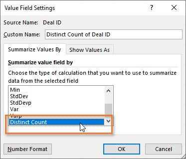
The Distinct Count function goes through the Deal ID column and gives us a count of the unique values, so our summary report will look just like it did for Solution #1.

Comparing the Two Solutions

Both of these solutions are great because they can be refreshed when new data is added to the source table.

The advantage to Solution #1 is that it can be done in any version of Excel. With that said, if you are running 2013 or later in Windows, Solution #2 is the superior option. This is because Solution #1 gets wonky when you try to filter the data down (say, for a certain product) or use slicers to dissect the data further.

If you'd like to learn more about using Pivot Tables, I have a separate blog post you can check out here: Introduction to Pivot Tables and Dashboards.

Other Solutions

There were lots of other great solutions to the challenge that were submitted. They included using Power Query and new dynamic functions. We will take a look at those in future posts, but I wanted to start with these two because they were more universal in terms of Excel version access.

If you have questions about either of these solutions, please leave a comment below!