Bottom Line: Learn how to quickly summarize bank statements that contain debit and credit columns with pivot tables.
Skill Level: Intermediate
Watch the Tutorial
Download the Excel Files
Feel free to download the workbook that I use in the video. I've included both the before and after versions for your convenience.
Use Excel to Summarize Your Statements
If you've ever wanted more out of your bank statements, such as summary reports by category or comparisons between incoming and outgoing funds, today's tutorial may be helpful for you. We are going to take a look at how Excel can help you analyze and summarize statements.
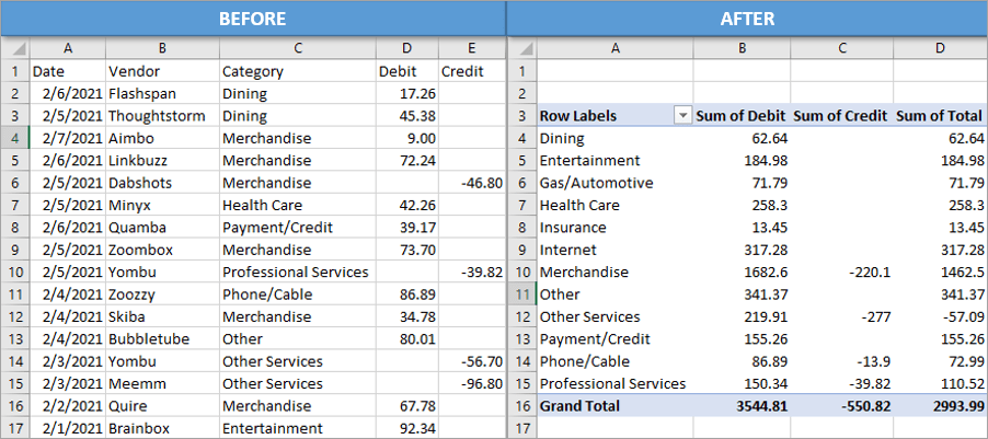
These could be statements for your bank account that show withdrawals and deposits. Or it could be credit card statements showing purchases and refunds. It could also be expense reports or any other type of statements that have debits and credits.
We'll learn how to create totals for those debits and credits and then make a summary report of the data using a pivot table.
Here's how.
Insert an Excel Table
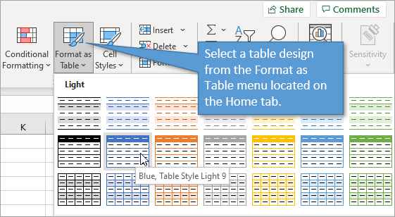
Beginning with statement data that you've imported from your bank or credit card company, the first step is to change the format of the data to a table.
With any cell in the data selected, go to Format as Table on the Home tab of the Ribbon. Then choose whatever color/design scheme you like best.
I've compiled 5 Reasons to Use an Excel Table as the Source of a Pivot Table to explain why we take this first step.
Insert the Pivot Table
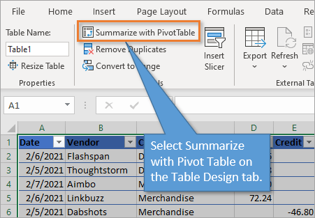
Start by selecting Summarize with Pivot Table, located on the Table Design tab. Then hit OK to put the pivot table on a new worksheet.
(If it's been a while since you've worked with pivot tables or your not familiar with them, you can check out my tutorial series here: Introduction to Pivot Tables and Dashboards.)
Create a Summary Report with the Pivot Table
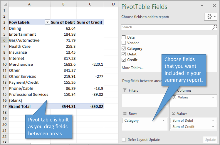
From here, we can build out our pivot table by dragging fields into the different areas of our table. I put the Category field in the Rows area. Then I added the Debits and Credits field to the Values area.
A natural question, once you have your debits and credits showing in your summary report, is how can I add them together? I'm going to show you two ways to go about that.
Option 1: Add a Calculated Field
With any cell selected in the pivot table, go to the Pivot Table Analyze/Options tab and open the Fields, Items, & Sets drop-down menu. Choose Calculated Field. This opens a window that allows us to create a formula for a field that will add the debits and credits together.
Name the field “Total” or whatever you like. Then create the formula by double-clicking Debit, typing the plus symbol (+) and double-clicking Credit. Then click Add to add this new field to the field list.
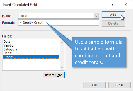
Note: This formula works when the debits are listed as positive numbers and the credits are negative in your table. If your data has those reversed, or both are listed as positive entries, simply adjust your formula as needed (changing the plus to minus, etc.)
When you hit OK, you will see the Sum of Total column added to the pivot table.
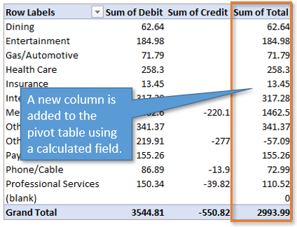
The great thing about this set-up is that it is really flexible for manipulating and changing. We can add or delete fields within the pivot table, or change the layouts and filters, and the calculated field will still work.
Option 2: Add a Calculated Column
For this option, we are making our adjustment to the source data range, not the pivot table itself. We'll add a column to the source table (I've labeled it “Amount”) and then create the same simple formula that adds the debits to the credits.
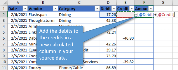
Because it's an Excel table, that formula will carry all the way down the column and give you the totals for each row.
Now that the column is added to the source data, you'll also see it in your list of fields to work with after you refresh the pivot table. (Keyboard shortcut for the refresh is Alt + F5.) Now you can move the new Amount field to the values area and see it appear in your pivot table.
Which is Better?
Both options give you the exact same results in terms of your pivot table. The calculated column method has a slightly better advantage in that the totals being added to the source data might be helpful if that data is also being used to create other reports, summaries, tables, or files.
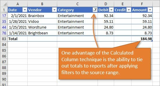
The calculated column is also useful for tying out numbers to the summary reports. You can filter the table and see the sum of the visible rows in the Total Row of the table.
Conclusion
One thing I wanted to mention is that you can remove the debit and credit fields from your pivot table and still retain the total column, if you wish. The table will still calculate accurately, whether those fields are actually showing or not.
I hope these solutions are helpful for you as you take a look at your bank or credit statements, so that you can quickly see what you are spending or saving in each category. If you have any questions or comments about this post, please feel free to leave a comment below.


Fha KS Rd
Thanks for this
How would you automate filling in the Category based on the payee value
Also could you use power query?
Hi Allister,
Great questions!
You could use a lookup formula like VLOOKUP or XLOOKUP to lookup and return the category based on a value. The lookup table would contain the list of values in one column and the categories in an adjacent column.
And yes, you could use Power Query for the lookups AND for creating the calculated column. In Power Query, the lookup is called a Merge. Here are a post and video on Merge in Power Query.
I hope that helps. Thanks again and have a nice weekend!
I really like your handouts. Keep it up. Thanks Jon
Thank you, Dickson. We appreciate your support!
Very simply explained. I got it! Thanks.
Thanks a lot
Hi John
A very interesting post, but my bank *.csv’s don’t come in this format.
They are usually, Number, Date, Account, Amount, Subcategory, Memo.
I normally use PQ and remove the number and account no.
I then add a conditional column based on the amount and call it credit or debit, the sub category can then be converted to whatever you need, Direct Debit, Card Payment etc, and the Memo field can be changed by replacing the text whatever suites eg Tesco shopping, ASDA Petrol etc.
You can then filter till your hearts content, then add a pivot table or whatever.
When the next month comes along it normally updates on it’s own as all the cv files are kept in one folder.
The CSV file are all in upper case, so once it’s processed and case is changed it’s easy to to find needed updates and change as required
Where are the templates?
Thanks, a mil, this helped a lot, as I’ve never done a Pivot before, but not sure how to interpret/sort the data, to match payments to debits, to see which payments don’t have corresponding debits or vice versa. The issue with my data is I inherited an account with several years’ worth of payments, with not enough debits to contra out the payments, so to try and pinpoint which payments (with debits coming much later and with some payments reversed out) is a tedious task to try and match, I needed excel to pinpoint payments that don’t have corresponding debits to clear them out, can’t seem to find a formula that works for this but I know Excel has one!