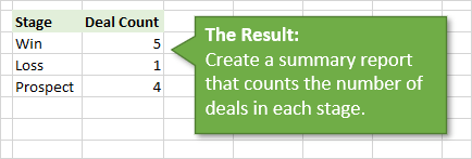
Bottom line: Create a summary report that counts transactions by a category when the data contains multiple rows per transaction.
Skill level: Intermediate
Video Explanation
Download the Excel File
You can download the Excel file that contains the source data for the challenge below.
The Challenge
This data analysis challenge is based on a great question from Rob, a member of our Elevate Excel Training Program.
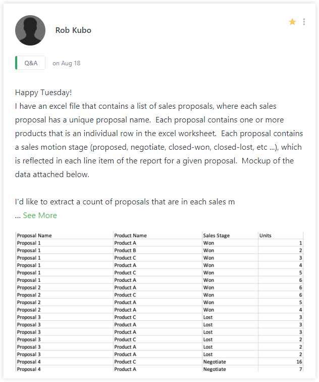
He has sales pipeline (CRM) data and wants to create a summary report of deal count by sales stage. The problem is that each deal/transaction has multiple rows in the source data. The data includes rows for each product in the deal.
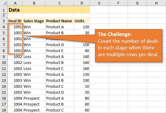
However, Rob only wants to count each deal one time in his summary report by sales stage. Here is an image of what the end result should look like.
Your mission, should you choose to accept it, is to use any of the tools or features in Excel to create the summary report.
Bonus Challenges
I have two additional challenges for you. These are not required, but do force us to think about making the report flexible and dynamic for future updates.
1. Account for New Data
Is it easy to include the new data in your results?
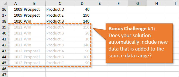
Your solution should be able to easily recalculate the results when new data is added to the source range. I put some additional data on the New Data tab in the workbook. You can copy/paste this below the original source data to test your solution.
We don't want to have to completely recreate the report every time the data is updated.
2. Account for New Sales Stages
What if the stage names change, or new stages are added to the system?
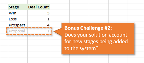
Currently, there are three stages (Win, Loss, Prospect). The data on the New Data sheet includes a new stage, Proposal. Your solution should also be able to automatically include this new stage in the results. Or include it without too much additional work.
Solutions
2 Ways to Calculate Distinct Count with Pivot Tables
How to Count Unique Rows with Power Query
Distinct Count Report with Dynamic Array Formulas
Share Your Solution
I love this question from Rob because there are A LOT of different ways to solve this problem in Excel. And of course, pros & cons to each.
However, I want you to give it a try! Don't worry about it being the “perfect” solution. That probably doesn't exist anyways…
You can leave a comment below or on the YouTube video with a brief description of the tools & techniques you used to solve the challenge. You can also upload your file to any cloud service like OneDrive, Google Drive, or Dropbox and post the share link in your comment.
I will follow-up with a video(s) explaining the most popular techniques and the pros & cons of each. We look forward to seeing your solutions and learning from everyone that participates. Thanks! 🙂


Assuming that all sales stages will be the same per Deal ID (i.e all win/loss etc)
Change the data set to a table
=UNIQUE(B4:B38) ‘to get the Stages
=INDEX(Table1[Sales Stage],MATCH(UNIQUE(Table1[Deal ID]),Table1[Deal ID])) ‘to get a list of win/loss/prospects
then
=IF(K4=””,””,COUNTIFS($O$4#,K4)) ‘ to count the results
I couldnt get the index & match to work inside the countif
It seems to work and will the extra data
https://1drv.ms/x/s!AomqbYFKl5QeivBUAYPqxZLtmrQdhg?e=ngpcDu
But now i have some work to do! Boring
First time i have ever commented on one of your posts so im going to start by saying, you are amazing. Learnt a lot from you.
Challenge accepted.
First thing to do is isolate the groups (Deal ID). This can be done using a new column (column E in this case) and adding a formula to separate the different values. first formula that comes to mind was an if formula.
‘=IF(A4=””,””,IF(COUNTIF($A$4:A4,A4)>1,””,”Yes”))’
I use the front part of the formula ‘=IF(A4=””,””‘ because i like my spreadsheets clean and tidy (OCD lol).
‘IF(COUNTIF($A$4:A4,A4)>1,””,”Yes”)’
this looks at column A and if the formula is dragged down, it will show a blank cell for every duplicate value.
Now in column E under the first unique Deal ID, you will get a yes.
the Deal ID can change from numbers to letters or mixed and you will get a yes regardless.
Now the counting part
‘=COUNTIFS(B:B,$H4,E:E,”YES”)’
Simple countif formula to count all the stages and all the yes’s.
the stage names can have new ones added or amended at a later date and the data stays in tack
new data can also be added at the bottom of the data set but the formulas need to also be added in column E.
my easy fix for this is to drag the formulas all the way down to a point where i wont need to add it until a later date in time.
sorry if i waffled.
Mario
Him Mario
My solution was very similar, but if you convert the data range to a table, you do not need to drag the formula down as the table automatically populates it for you 🙂
Very true, I’m use to not working with tables, but queries which do it automatically lol
Tables rock! I probably overuse them
Change data to Table>Create Pivot ensure you check add to Data Table; make pivot and change value to district count. Adding bonus data to the data table after refresh will update automatically.
This was my first attempt but I couldn’t find the district count. Forgot to add to data model. 🙂
Used the group by function in power query.
Step 1: convert original data to excel table.
Step 2: use powerpivot to load data into data model
Step 3: create pivot table using powerpivot using sales stage as rows and distinct count of deal ID as values. This is the end result.
Bonus answer:
– when you add another stage, or change any part of original data, you need to hit refresh of your data model. this will update your results.
– appending new data to the original data and hitting refresh of data model will also update your results.
Turn Data into an Excel table
Summarize with a Pivot Table
Check Add this to the data model
Pivot Table
Row – Sales Stage
Values – Deal ID – Summarize Value field by Distinct Count
I was going to whip up a VBA sub routine; but this is more elegant and simple to use in my opinion. In the Results WS:
A B
1 Result
2
3 Stage Deal Count
4 Win =SUM(–(UNIQUE(Data!A:B)=A4))
5 Loss =SUM(–(UNIQUE(Data!A:B)=A5))
6 Prospect =SUM(–(UNIQUE(Data!A:B)=A6))
I hope I rendered the picture. There is no limit for the data added to the original source and the formula above can be easily dragged in Column B according to the criteria set in column A (ie a different Stage added or changed).
The only problem I see is that if the structure of the data changes, one will get bad results. Say, deal 1001 had just 1 stage that is inconsistent, we would be mislead. I didn’t guarantee for the correctness and the correction of the data set.
With a sub, the latter concerns can be dealt with in a way or another… ehh coding always makes things more complete 🙂
Get Data from Table > Remove Duplicates on Deal ID. Close and Load Pivot Table. Adding bonus data to the data table will automatically update after refresh.
I changed data to Table, added one columne with formula =IF([@[Deal ID]]-A5>1000;-1;[@[Deal ID]]-A5) (to distingues between new deals) and count results with conditions below.
Adding new data just works immideately, for new category just need to expand table with results.
=IF(H4=B4;COUNTIFS(Tabela1[Sales Stage];H4;Tabela1[A];-1)+1;COUNTIFS(Tabela1[Sales Stage];H4;Tabela1[A];-1))
My solution starts with making the data into a table. Then I get the unique Stages with
=UNIQUE(Table1[Sales Stage])
In cell L1 I entered this formula:
=UNIQUE(Table1[Deal ID]&Table1[Sales Stage])
which gives the unique combinations of Deal and Stage. So it looks something like
1001Win
1002Loss
etc.
Then in cell I4 (First Deal Count), I entered:
=IF(H4=””,””,SUM(1*ISNUMBER(FIND(H4,$L$1#))))
and filled it down 50 rows (or 2000, depending on your real data)
This does the whole job, and works when you append the new data.
To make it look nicer, I hid column L.
As per Jim Williams a Pivot Table is a quick and easy option with Sales Stage as the row item and Deal Count in Values (with field setting changed to ‘Distinct Count’). This will update when new data is added but requires the user to refresh the data in the pivot table.
I suspect there is a more elegant solution using UNIQUE etc. but I was struggling to write a formula that would give you a combination of a count of Sales Stage with unique deal references.
I think I’d try two array formulas, but unfortunately, I don’t think they’re compatible with older versions of Excel:
Stage column:
{=UNIQUE(INDIRECT(“B4:B”&MATCH(2,1/(A:A””))))}
Deal Count column (and copied down):
{=SUMPRODUCT(–(COUNTIFS(INDIRECT(“$A$4:$A$”&MATCH(2,1/(A:A””))),UNIQUE(INDIRECT(“$A$4:$A$”&MATCH(2,1/(A:A””)))),INDIRECT(“$B$4:$B$”&MATCH(2,1/(A:A””))),L4)>0))}
https://1drv.ms/x/s!Av-Y102dP161gcH9Uoh_zB82zqf36s8?e=8kgk7x
I used formulas to solve the problem.
Create a unique list
=IFERROR(INDEX($B$4:$B$5000,MATCH(0,COUNTIF($N$2:N2,$B$4:$B$5000),0)),0)
Attach the list to data validation
=OFFSET(Data!$N$3,0,0,COUNTA(Data!$N$3:$N$13)-COUNT(Data!$N$3:$N$13))
use countif to count the result.
=COUNTIF(Data!$B:$B,Results!$A4)
you can append more data and stages the solution will pickup in data validation list.
Just one DA formula for both the Stages and Deal count columns including also a grand total:
=LET(data1,Data!$A$4:$B$1000,
data2,Data!$B$4:$B$1000,
r,FILTER(UNIQUE(data2),UNIQUE(data2)0),
nb,ROWS(r),
a,TRANSPOSE(–(FILTER(UNIQUE(data1),{0,1})=TRANSPOSE(r))),
deal,MMULT(a,SEQUENCE(ROWS(FILTER(UNIQUE(data1),{0,1})),,1,0)), IF(SEQUENCE(nb+1)>nb,CHOOSE({1,2},”Total”,SUM(a)),CHOOSE({1,2},r,deal)))
Here’s the file:
https://www.dropbox.com/s/b0iln9blps51ts1/data-analysis-challenge.xlsx?dl=0
I had the same solution as Jim, create a pivot table, add it to the data model, make the pivot, with a distinct count of Deal ID. No VBA and associated challenges in sharing a VBA enable workbook, super easy to update by clicking refresh. Less than 5 minutes to build.
I firstly used a helper (&) to combine the Deal ID and Sales Stag. I copied them to another cell and paste as value after which I removed duplicate. Then I used COUNTIF and MID function to arrive at my result.
https://drive.google.com/drive/u/0/my-drive
I unfortunately don’t have time to attempt this right now, but I would definitely use Power Query to handle this, grouping the rows by deal number. Then load the results to a very simple pivot table with stage in rows and count in values. You could skip the power query by just pivoting the original table and using distinct count, but I think you could update with new source data much more quickly if you used PQ.
Make sure that the data is formatted as a table. Select the entire table and insert a pivot table AND make sure to select “Add this data to the Data Model” at the end of the pop-up window. This step allows categorical data to be manipulated as quantitative data. Select where you want the table on the spreadsheet. In the pivot field chooser select “Sales Stage” in ROWS. Select “Deal ID” as VALUES, but when selecting the Summarize Value Field scroll all the way down to “Distinct Count” and voila. It should update as long as your spreadsheet is connected to the data source. Might need to manually refresh spreadsheet upon new data or put a macro in to auto-update when table is changed, but the hard part is done 🙂
Convert data to a table (named “tData”)
On Results tab:
Add formula to A2: =UNIQUE(tData[Deal ID] & tData[Sales Stage])
Under Stage heading of results table (cell C4), add formula to give unique Stages: =UNIQUE(tData[Sales Stage])
Under Deal Count heading of results table (cell D4), add formula to give required count: =COUNTIF(A2#,”*”&C4#)
Hide column A
Adding extra data to tData will achieve both bonuses
This is better than mine because it is more flexible.
Hi Jim,
had the same approach but without a helper column:
=SUM(1*(RIGHT(UNIQUE(tData[Deal ID]&tData[Sales Stage]);LEN(C4))=C4)) and couldn’t get that to work with the spillover correspondingly to your CountIF(A2#).
Any idea why?
Hi Jim, I had a very similar approach, however, as per Ralph’s response, the formula in the ‘Deal Count’ column does not spill down (for Jim and me at least!).
To get around this (in case of extra stage types being added) I:
– copied the formula in ‘Deal Count’ down 10 rows
– made it clear via formatting that the data only ran for 10 rows (of course, pick any number of rows as needed – eg if we know there will only ever be 5 stages, pick 5 rows)
– wrapped the formula in an IF statement to only show if there is data in the ‘Stage’ column eg:
=IF(ISBLANK(A4),””,COUNTIF($C$4#,”*”&A4&”*”))
(NB also note the use of $ to make C4 absolute, else the formula copies down incorrectly)
Hi Duncan,
It DID fill down for me, but not when I tried to combine the helper with the Deal Count formula to give a single-formula solution (as per Ralph’s experience)
I still prefer this solution to a Pivot Table / Power Query solution preferred by the majority of other posters
To me, it seems simpler and doesn’t require a Refresh
If making the data into a Table is to be avoided (can’t think why, but it may be a requirement of Jon’s challenge not to alter the original format), it would be possible to do it old style with dynamic ranges, which used to be the norm before Excel 2007 (I’ve rarely needed to use them since and don’t miss them!)
So, I realised my error, I forget to add the spill ‘#’ (still new to these spilling formulas!). To confirm, as you had it:
=COUNTIF(C4#,”*”&A4#)
DOES spill. Sorry about that!
For me also, if I try and replace ‘C4#’ in the above formula with the formula IN cell C4:
UNIQUE(tblDeals[Deal ID]&tblDeals[Sales Stage])
(so that there is no need for the helper formula in cell C4) then Excel complains, saying there is an error in the formula. SeemS that COUNTIF doesn’t like it (other formulas eg LEFT/MID seem fine when I tested them)
So stumped on that one!
Here is my solution
https://www.dropbox.com/s/9ri0ylzw5t84bvk/Data-Analysis-Challenge.xlsx?dl=0
Hi Jon,
1. I made the original range a table, in order to be completed with new data.
2. Instead of hard coding the elements, I made a unique list of the column “Sales Stage” with the array formula =IFERROR(INDEX(Table2[Sales Stage]; MATCH(0;COUNTIF($G$1:G1; Table2[Sales Stage]); 0));””)
3. I also inserted the results range to a table
4. I added a helper column to the original table, where I use the formula =IF(A3=[@[Deal ID]];1;0) (where [@[Deal ID]] is A2).
5. And finally in the deal count I put
=COUNTIFS(Table2[Sales Stage];[@Stage];Table2[helper];0)
6. seems to be working on update
Something between Daniel’s and Bob’s solutions. Doesn’t require LET (which I haven’t got yet) or a helper column…
1. Convert the Data range into a table.
2. In cell H4: =UNIQUE(DataTable[Sales Stage])
3. In cell I4: =SUM(–(XLOOKUP(UNIQUE(DataTable[Deal ID]), DataTable[Deal ID], DataTable[Sales Stage]) = $H4))
4. Drag formula from I4 down as many rows as you ever expect to need for new stages.
Oops… the web page converted my double minus, after “SUM(“, into a long dash.
I’ve added a pivot table making sure I added the data to the “Data model”. In that way I can summarise the deals/stage with Distinct count.
Also you would need to turn your data into a Table so any new data you add would pull through when the pivot is refreshed
https://drive.google.com/file/d/14V4bE6CR5tDzZ2yu44j3KFPYncv6_g3S/view?usp=sharing
Use Power Query to load the data range into the Power Query Editor. Select the Sales Stage column. Click the Group By icon. Set the New column name to Deal Count, Operation to Sum, and Column to Units. Click OK. Close and Load to the Results tab. For new data, add to the bottom of the table and click Refresh All.
https://www.dropbox.com/s/nwf98gmvau0lk2g/data-analysis-challenge%20result.xlsx?dl=0
create a query – get data form existing workbook – group by stage, Deal ID with sum on Units -on the result Group by Stage to Count Deal Ids – and then load it to the “Result” worksheet. thanks Jon
I did a Power Query on the data where I removed unnecessary columns and removed duplicates. I then created a pivot table with a count of the Deal ID and sorted the data Z to A. All new data updates correctly after refreshing both the power query and the pivot table.
I was going to whip up a VBA subroutine but decide that this solution is more elegant and simple to use in my opinion. In the Results WS:
Enter in A4 “Win”. Complete with the other criteria you need under A4.
Enter in B4 “=SUM(–(UNIQUE(Data!A:B)=A4))”
Drag the formula down to the last criteria.
-DONE
I hope I rendered the picture. By adding data to the original source the values get updated and one can add criteria and simply drag the formula in the B-column down where necessary.
However I am assuming that the data retains its structure and logic at all times. I did not account for inconsistencies (say the second win for 1001 turns to a loss). I cannot guarantee for the correctness of the data and its corrections. With a sub these can be taken care of in a way or another… ehh coding is always somewhat more complete 🙂
Simple Power Query…
1. Make data range into table.
2. Make PQ from this table. (Data > From Table/Range)
3. Deal ID column: Remove Duplicates
4. Sales Stage column: Group By… (accept default parameters)
5. Close & Load
Of course, with a PQ you will have to refresh every time you update the input data.
Nice to able to finally try one of these challenges.
My (independent) answer was essentially the same as Richards:
.Step # Tool Description
1 Excel Convert Data to table
2 Excel Give table descriptive name
3 Excel load data to PowerQuery
4 PQ Select Deal ID and Sales stage
5 PQ Remove duplicate rows
6 PQ close and load to PivotTable on Results tab
7 PT Pivot Rows on Sales stage
8 PT Pivot Count on Sales stage
9 Excel Define custom sort order on stage
10 PT apply custom sort order to Pivot
Done, about 10 minutes (had to do a little playing around to find a couple of thing)
Bonus 1- add data
Copy new data to bottom of data input table
Right click on Pivot, select refresh
Done: < 1 minute
Bonus 2: new categories
automagically handled by PQ and PT
Here is my example file
https://1drv.ms/x/s!Am8lVyUzjKfppCSFlMm_MPqdLkd5?e=pEgtpJ
This is much simpler than the complex formulae that I used. Thanks.
Hi Richard, I had a formula solution, but your answer does it for me. And I learnt 2 new things in PQ:
– you can remove duplicates across 2 columns by highlighting them first (presumably works with more columns too)
– the whole “Group By” functionality
Thanks!
(NB I guess if you wanted to “bullet-proof” it so there’s absolutely no extra work needed by the user (ie refreshing the query) you could add a little VBA to auto-refresh the PQ data every time the ‘Results’ tab is selected?)
Select the source data, change to table – ctrl T. Create a pivot table from the data table, check the box – “Add this data to the Data Model. Use the Sales Stage for the Rows, and then use Distinct Count for the Deal ID.
Transforming the data to a table will automatically add any new data added to the bottom of the table. And update the pivot table.
Convert the data to a table.
Add a column in column E titled Deal count.
In cell E4: =IF(COUNTIFS(B$4:B4,[@[Sales Stage]],$A$4:A4,[@[Deal ID]])>1,0,1).
In cell I4 I used: =SUMIF(Table24[Sales Stage],”WIN”,Table24[Deal count]) to count the stage. Drag the formula down, changing the “WIN” to the other stage names.
I also did the results in a pivot table (Sum of Deal Count).
I am partial to a simple power query.
1. Turn data into a table.
2. Get & Transform from Table
3. Delete Product and Units columns
3. Remove duplicate rows
4. Group with Count Distinct
This is easily done from the menu, but the code created looks like this:
let
Source = Excel.CurrentWorkbook(){[Name=”Table1″]}[Content],
#”Changed Type” = Table.TransformColumnTypes(Source,{{“Deal ID”, Int64.Type}, {“Sales Stage”, type text}, {“Product Name”, type text}, {“Units”, Int64.Type}}),
#”Removed Columns” = Table.RemoveColumns(#”Changed Type”,{“Product Name”, “Units”}),
#”Removed Duplicates” = Table.Distinct(#”Removed Columns”),
#”Grouped Rows” = Table.Group(#”Removed Duplicates”, {“Sales Stage”}, {{“Count”, each Table.RowCount(Table.Distinct(_)), Int64.Type}})
in
#”Grouped Rows”
Create data source from Data sheet columns A:B. Use Power Query to transform (delete top 2 rows, make new top row –> field names, and then delete duplicate rows). Close and export as pivot table. Adding or modifying Data sheet works after a refresh.
Transform the dataset into a table. Make sure each field is named. Enter, say in F11: UNIQUE(Sales_Stage). Enter, say in H22: =UNIQUE(Deal_ID:Sales_Stage). Alongside the results in F11, in G11, enter =COUNTIF(H22#,F11#).
Steps
1. Converted Data to a table.
2. Uploaded table to the data model
3. Created a measure using DISTINCTCOUNT(Table1[Deal ID])
4. Created a pivot table using data model with Sales Stage in rows and my measure in values.
5. Added extra data from the New Data tab and pivot table updated with new Stage and new count.
I used the Data/Advanced Filter to get unique values on the data page and then, on the results page, I used COUNTIF to compare those data values with the result row values (win, loss, prospect).
Roger ( Belgium )
i have two solution
a pivot table from a data model using distinct count
power query and grouping by
file in the link below
https://drive.google.com/file/d/1WreBk5OaHeNRLqVjwyF7fzmiEQu9dCcu/view?usp=sharing
Convert the data to table
Copy and paste sales steage in result sheet say in column D
Remove duplicate
In column E use, =COUNTIF(Table1[Sales Stage],Results!D3)
The copy new data and add to data sheet after last row
In result sheet type Proposal immediately after Prospect and count for Prospect will automatically show.
Use the link below to view my solution
https://drive.google.com/file/d/1dYoynpz3dUV3sLQo_A8qzG_BPcgm5pJt/view?usp=sharing
Hi Jon,
I will solve the issue by using Pivot Table. I will put the data in a table format by using a shortcut key, Ctrl T and named the table. By doing so, when we refresh the Pivot Table, results will update new data added as well.
Basic Overview: Use Power Query to Group
1) Select data and Insert Table
2) Add a New Query from Table
-Group by Sales Stage and Product Name
-Group by Sales Stage
-Rename Columns
let
Source = Excel.CurrentWorkbook(){[Name=”Table1″]}[Content],
#”Changed Type” = Table.TransformColumnTypes(Source,{{“Deal ID”, Int64.Type}, {“Sales Stage”, type text}, {“Product Name”, type text}, {“Units”, Int64.Type}}),
#”Grouped Rows” = Table.Group(#”Changed Type”, {“Sales Stage”, “Deal ID”}, {{“Count”, each Table.RowCount(_), type number}}),
#”Grouped Rows1″ = Table.Group(#”Grouped Rows”, {“Sales Stage”}, {{“Count”, each Table.RowCount(_), type number}}),
#”Renamed Columns” = Table.RenameColumns(#”Grouped Rows1″,{{“Sales Stage”, “Stage”}, {“Count”, “Deal Count”}})
in
#”Renamed Columns”
RESULT 1:
Stage Deal Count
Win 5
Loss 1
Prospect 4
4) Add New Data to row below Data table
5) Refresh Query
RESULT 2:
Stage Deal Count
Win 7
Loss 2
Prospect 4
Proposal 1
Simple and elegant 🙂
1) Convert range to a Table.
2) Add column to table called “RowCount”
3) In first row (in this example, row 4), enter the formula
“=IF(COUNTIF($A$3:A4,A4)=1,1,0)”
4) Create a normal pivot table.
Rows = Sales Stage, Values = (sum of) RowCount
5) Refresh pivot each time data is added to Table.
As data is added, Rowcount column formula automatically copies down to the next row in the table and the pivot table automatically expands to include any new Sales Stages.
Similar to Richard’s solution
1. Make the data range ionto a table
2. In the Results tab, set the Deal Id to =UNIQUE(Table1[Deal ID])
3. Set Stage to =VLOOKUP(A2,Table1[[Deal ID]:[Sales Stage]],2,0)
(I’m not happy with this one because you have to extend the range for the new Deals)
4. For the Summary, where the Stage is in B and the desired stage name is in D
COUNTIF(INDIRECT(“b2:b” & 1+ROWS(UNIQUE(Table1[Deal ID]))),D2)
The difficulty with this is that you need to manuially extend the Stage range for each new deal and the summary for each new stage.
I’ll think about this some more.
Revision
1. Same as above
2. In the Results tab, Set Del Id =UNIQUE(Table1[[Deal ID]:[Sales Stage]])
3. For the summary, set Stage to =UNIQUE(Table1[Sales Stage])
4. same as above and you don’t need to change anything manually until you add a new stage. In which case, you just copy the formula in E down.
Nice challenge! Two solutions, both expandable and refreshable as they build on a table:
Create Table:
1. click on the data and CTRL+T to tranform it to a table.
2. Name the Table e.g. “Data”
3. On the Data tab click From Table/Range to bring it to Power Query.
Power Pivot:
1. Load the query to the Model (only connection)
2. Build a pivot with Sales Stage in the row area
3. On the Power Pivot tab click Measures to create New Measure:
DISTINCTCOUNT(Data[Deal ID])
4. Bring the measure to the value area.
Power Query:
1. Reference your “Data” query
2. Group by Sales Stage using Count Distinct Rows
3. Load the query as table to any sheet
let
Source = Data[[Deal ID], [Sales Stage]],
#”Grouped Rows” = Table.Group(Source, {“Sales Stage”}, {{“Count”, each Table.RowCount(Table.Distinct(_)), type number}})
in
#”Grouped Rows”
Refresh:
Plenty of options, but probably the easiest in this case is with a right click on the pivot or the table.
Hope the explanation was clear enough. If not, please let me know.
Now I am curious on the other solutions!
On Results sheet
I used named ranges (dynamic) defined below
deal=OFFSET(Data!$A$4,0,0,COUNTA(Data!$A$4:$A$100))
stage=OFFSET(Data!$B$4,0,0,COUNTA(Data!$B$4:Data!$B$100))
H4 =UNIQUE(stage)
I4 =IF(H4=””,””,COUNTA(UNIQUE((FILTER(deal,stage=H4)))))
copy down as many rows as stages expected
I just use the simple pivot table.
Rows for ID and product name
Values for Units change the value field to count
Change report layout to show in tabular form and add subtotal for Deal ID on the bottom of the group
I think, finish in 5 minutes. Hope it serve the purpose.
Convert data to table
Power Query – get data from table/range
Delete Product name and units column
Remove duplicates from Deal Id Rows
Group by Sales Stage Column
new column = Deal Count
Operation – Count Rows
close and load to sheet as table
add new data to data table and refresh
On the DATA tab:
Convert Range to Table (Table_Data)
Select Columns A:D
On the RESULTS tab:
Insert Pivot Table
Use (able_Data as Source
CLICK ADD THIS DATA TO THE DATA MODEL
Rows = Sales Stage
Values = Deal ID
Value Field Setting > Distinct Count
This solution accounts for all changes in the data.
1. Convert the data into table
2. use the formula with combination of CountA,Unique & Filter against each of stages Win, Loss & Prospect.
COUNTA(UNIQUE(FILTER(Table1[Deal ID],Table1[Sales Stage]=H10)))
A quick solution and simple.
1 Convert the data to a table
2 In the import data add this data to the model
3 Create a pivottable canvas
4 Drag fields Sales Stage to rows and field Deal ID to values
5 Change Deal ID values field setting to Distinct Count.
In my solution I have added a Sales Stage slicer refresh the workbook and the report show all unique values.
https://drive.google.com/file/d/1sgwyVAr9U3cSvCTeDqRmhIuuZeiSB6K8/view?usp=sharing
Dear Jon,
Please find the enclosed file for the Data Analysis Challenge.
Just a Pivot got me the result. And the New Data converted to Data Table so if any data added can get into Pivot table.
And Pivot table is on Auto refresh when ever file is open data will be updated.