Bottom Line: Use Power Query to count distinct rows in a data set that contains multiple rows per transaction, invoice, etc.
Skill Level: Intermediate
Video Tutorial
Download the Excel File
You can download the example file from the video here. I've included both the original file and the file with the solution:
Solving the Data Analysis Challenge
This post and video are the second in a series featuring solutions to a challenge I posed to readers. The inspiration for this data analysis challenge came from Rob, one of our Elevate Excel Training members.
The challenge is to create a summary report of deal count by sales stage. The issue is that there are multiple rows for each deal (transaction) in the source data. So we need to find a way to just count the unique rows for each deal.
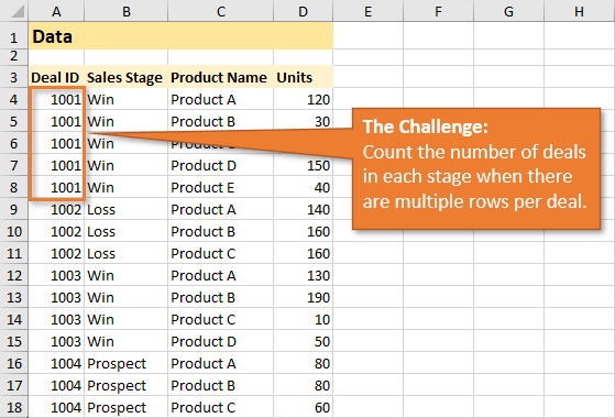
To see the first set of solutions to the challenge, using Excel Tables and Power Pivot, watch this tutorial: 2 Ways to Calculate Distinct Count with Pivot Tables. Today, we're going to solve the same challenge using Power Query.
A quick shout-out of thanks to everyone who submitted a solution to the challenge! Excel Campus viewers are the best!
Use Power Query to Get a Distinct Count
Let me start by noting that Power Query is available only to those who are running Excel 2010 or later for Windows. If that's not you, I suggest using the pivot table solution I mentioned above.
For the Power Query solution today, the first step is to format the data as an Excel Table.
To do that, just select any cell in the data set, and click on Format as Table on the Home tab. Right-click on the table format you want and select Apply and Clear Formatting.
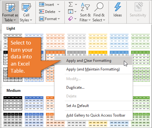
Hit OK when the Format as Table window appears.
Now that the data is formatted as a table, you can go to the Data tab and click on the From Table/Range button in the Get & Transform Data section.
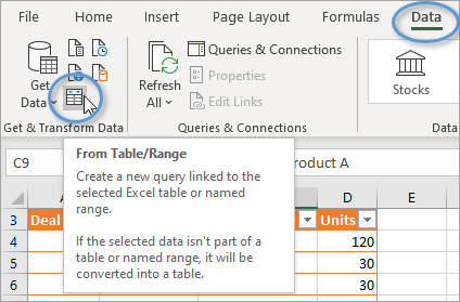
Note: On Excel 2010 and 2013, Power Query is on it's own tab. Please see my post on how to install Power Query if you are on one of those versions of Excel.
This opens up the Power Query Editor, loading a preview of our data. From here, we really only need to do two things:
1. Remove Duplicates
Since we want to remove the duplicates in our data set based on both the Deal ID and Sales Stage columns, we will select both columns before getting rid of the duplicates. With both columns selected, you can right-click on either of them and choose Remove Duplicates.
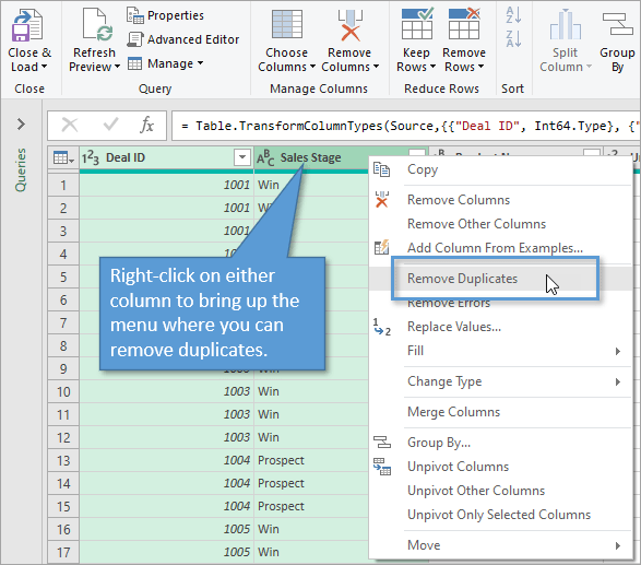
When multiple columns are selected, Remove Duplicates will look for duplicates by combining the values in each row from the selected columns. The result is a list of unique combinations of the Deal ID and Sales Stage columns.
Note: Technically we don't need to select two columns because the Sales Stage is always the same for each Deal ID in this example. Therefore, you can select the Deal ID only and Remove Duplicates. However, you might have a scenario where there are different stages per Deal, and in that case you would want to select both columns.
2. Find the Count
From the remaining data in our data set, we want to count up each entry in the Sales Stage column. To do this, we can use the Group By feature in Power Query. With just the Sales Stage column selected, click on Group By, found on the Home tab in the Ribbon.
In the Group By window, we can use the Basic settings that are already there by default.
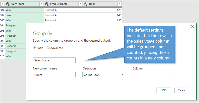
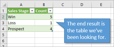
That essentially leaves us with the report we are looking for because Power Query has added the number of entries for each Sale Stage and presented them as a count in a separate column.

If you click on the top half of the Close & Load button, it will export that new report as its own new worksheet in the workbook.
Pros and Cons for Using Power Query
One great thing about using Power Query is that as we add or delete source data entries, we can refresh the output table ( Alt + F5 ) to include those changes.
Another advantage of using Power Query is that your source data does not have to be an Excel worksheet. You can import data to Power Query from a database, website, .CSV file, or other source.
A disadvantage to this method is that you lose the ability to filter down further by other columns, such as Product. For that type of flexibility, the pivot table method is better.
Conclusion
In my next post, we will take a look at solving the data analysis challenge using Excel's new dynamic array formulas, which are always fun to work with. Until then, let me know if you have any questions about this solution that uses Power Query by leaving a note in the comment section below.


Add comment