The Most Dangerous XLOOKUP Argument

Bottom Line: Avoid using a certain argument in XLOOKUP without proper investigation to prevent errors and ensure accurate data retrieval.

Skill Level: Intermediate

Watch the Tutorial

Download the Excel File

You can follow along using the same Excel file that I used in the video.

XLOOKUP is a powerful function in Excel, but it has one feature that can cause problems if not used correctly. In this blog post, I'll highlight that feature and share some best practices and habits to help you avoid potential issues.

Writing the XLOOKUP Formula

To demonstrate this common mistake with XLOOKUP, let's write an XLOOKUP formula.

In our example, we have some ticker symbols in a portfolio table, and we want to look them up in another data set to return the price. We'll use XLOOKUP for this.

1. Start typing =XLOOKUP, then tab into that.
2. Select your lookup value (the ticker symbol), then press Ctrl+Shift+↓ to select all the way to the bottom. Hit F4 to make that an absolute reference.
3. Move on to the return array, which will be the price. Again, use Ctrl+Shift+↓ and F4 for the absolute reference.
4. For the if_not_found argument, we'll return a blank with two quotation marks, then hit Enter.
5. Double-click the fill handle to copy the formula down.

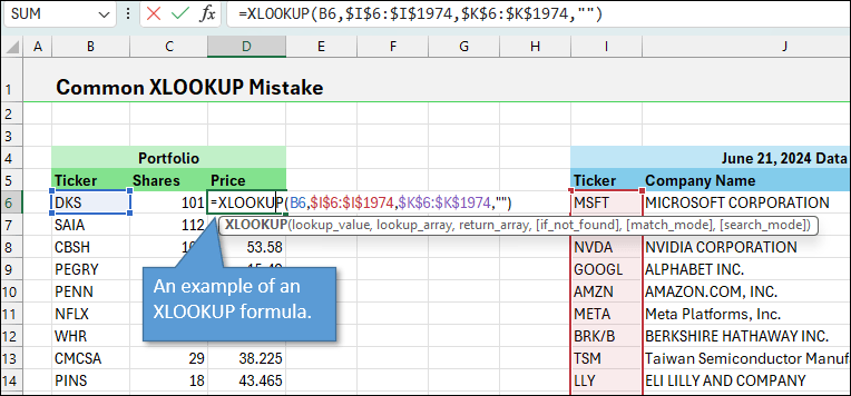
If writing this formula causes confusion for you, feel free to take a step back and check out these tutorials that explain XLOOKUP formulas in more detail:

• The New XLOOKUP Function for Excel
• Shortcuts for Writing XLOOKUP and VLOOKUP Formulas
• How to Fix & Prevent the #VALUE Error with XLOOKUP

Identifying Common Errors

You'll notice some blank cells, which might be because not all ticker symbols exist in the other table. However, there could be other reasons.

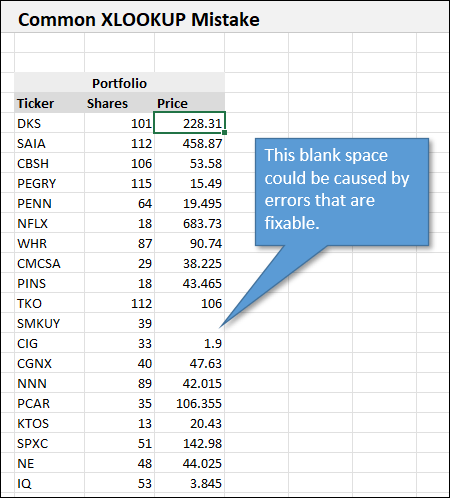
A common mistake is specifying the if_not_found argument without investigating the cause of the error. This argument handles any errors, so if there's a mismatch or Excel can't find the value, it returns what we specify in if_not_found.

Many users get in the habit of specifying this without investigating.

Best Practice for Using if_not_found

A good habit is NOT to specify if_not_found first unless you're diligent about investigating blank cells. Since it's an optional argument, you can leave it out. After copying the formula down, errors will stand out more, prompting you to investigate.

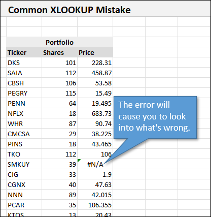
Investigating Errors

To investigate, copy the ticker from the row that has the error (Ctrl+C), and open the Find window using Ctrl+F. Paste the value and search within the ticker column of the source data.

If the value is there but has an extra character like an asterisk or space, XLOOKUP won't find it due to the exact match requirement. Cleaning up these characters is crucial.

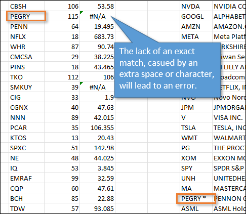
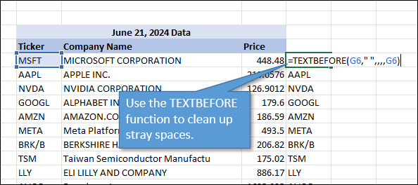
If you have tickers with extra spaces, use the TEXTBEFORE function to clean them up. The text to evaluate is the ticker symbol, and the delimiter is a space. If it doesn't find a space, it returns the ticker. Double-click the fill handle to copy the formula down, and your data is cleaned up.

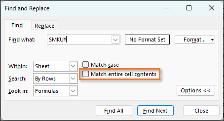
If there's still an error, gut-check it with another find operation to ensure no matches exist. Ensure “Match entire cell contents” is unchecked in the Find Options for a more thorough search.

Adding Error Handling Back to XLOOKUP

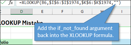
After investigation, you can add the error handling back to XLOOKUP. Specify the if_not_found argument, such as returning a blank or a custom message. This ensures errors are handled appropriately after thorough investigation.

XLOOKUP Trivia

An interesting piece of trivia: XLOOKUP was the first function to receive error handling with the if_not_found argument. Previously, we used the IFERROR function with VLOOKUP or INDEX MATCH for error handling. XLOOKUP's built-in error handling cleans up formulas and makes them easier to read. However, it's essential to use it correctly, with proper investigation to avoid issues.

Conclusion

Hopefully, this post helps you prevent errors with your XLOOKUP formulas. I'm curious to know if it's helpful for you or if you have other tips for preventing errors. Leave a comment below and let us know.

I mentioned in the video that you can subscribe to my free newsletter. Click here to do that.

And if you're wondering why I didn't use Excel tables, check out this video where I explain why. Thanks for reading. Have a great day!