Bottom Line: Learn the most common error with XLOOKUP and how to fix it.
Skill Level: Beginner
Watch the Tutorial
Download the Excel File
#VALUE! Error
When working with XLOOKUP functions, there are two main errors that I've encountered, and both can be avoided using the same solution. Let's look first at the #VALUE! error.
When you see a #VALUE! error in your XLOOKUP function, the most likely reason is that your lookup array and your return array are not the same size.
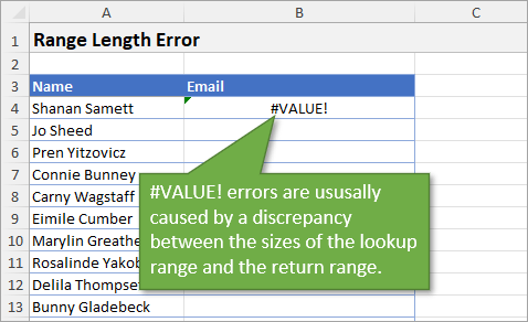
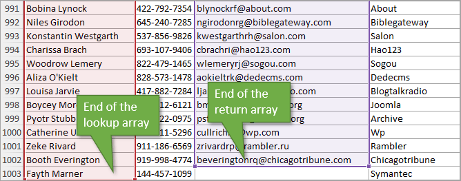
In my example, the reason the arrays are different sizes is that there is a blank cell at the end of my return array. When I wrote the formula, I used the Crtl + Shift + ↓ shortcut to jump to the end of my column, and that last blank cell wasn't part of the selection.
As you can see, my lookup array ends with row 1003 while my return array ends with 1002.
The Crtl + Shift + ↓ shortcut is one that I covered in my last tutorial: Shortcuts for Writing XLOOKUP and VLOOKUP Formulas.
Before we talk about a solution, let's look at another error you might encounter: the Absolute Reference error.
Absolute Reference Error
This error isn't indicated by a # prefix. It's noticeable from mistakes in the returned results.
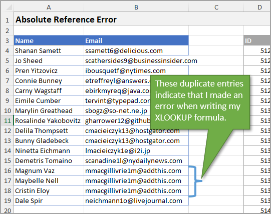
The reason for the error is that I forgot to hit F4 to make my values absolute when I wrote my XLOOKUP function. This can happen when writing either the lookup range reference or the return range reference, or both.
The Solution: Excel Tables
The solution for both of these errors lies in making your data set into an Excel Table. By using an Excel Table, your columns will always be the same size and your references will always be absolute.
To change a table into an Excel Table you can use Ctrl + T or use the Format as Table button on the Home tab of the Ribbon.
Once your data is converted to an Excel Table, you can use the keyboard shortcut Ctrl + Space to select the entire column when writing your lookup formula.
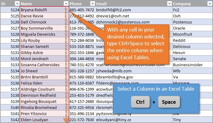
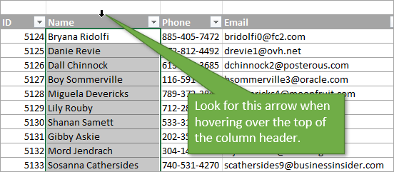
If you prefer to use your mouse instead of a keyboard shortcut, you can hover your mouse over the top of the column header until your cursor becomes a small down arrow. Then left-click to select the column.
Conclusion
For a succinct but helpful overview of XLOOKUP, check out this post: XLOOKUP for Excel: Explained in 3 Minutes.
And if you're not sure when to use VLOOKUP instead of XLOOKUP, you can watch this tutorial: XLOOKUP vs. VLOOKUP.
If today's post about lookup formula errors was helpful for you, if you have questions, or if your XLOOKUP is returning other errors/incorrect results, leave a comment and let us know.


Rather than selecting an array and making an absolute reference, why not just select the entire column? You don’t need to be in a table to select the entire column. What am I missing?
Hi Cary,
Great question! These are typically referred to as whole column references. I was going to cover them in this post/video, but decided to do a separate video on this topic.
There are a few risks to using whole column references.
They have the potential to slow down the calculation speed of your file and can produce incorrect results if you or other users of your file accidentally add data below the used range.
I’ll cover the pros & cons in more detail in the upcoming post.
I hope that helps. Thanks again and have a nice day!
Hello, What if you get the error #n/a “Error
Array arguments to XLOOKUP are of different size.” but the values are the same example: =xlookup(importxml(“sheet_url”,”sheet1!A3:A”),importxml(“sheet_url”,”sheet1!B3:B”),””)
we have several columns of formulas similar to this importing data from other sheets and as of the last few days they are not working in some columns. There is text in all of the cells of A:B
Hey Jon, I definitely like the table approach, especially as the tables are dynamic. Another method I have been using is by columns ‘xlookup(M1,B:B,D:D,””)’. Is this OK to use or could it be problematic?
Hey Craig,
Great question! These are referred to as whole column references. Cary had the same question on this post. Check out my reply to Cary to see some of the potential issues.
I’ll be covering this in more detail in an upcoming post.
Thanks! 🙂
I work a lot with Excel files which were exported by an ERP system. The structure is not very consistent, sometimes columns are shifted or deleted. and there is not ascending or descending order.
My favorite function threfore are combinations of Offset and Match, so I can find a specific header, then the row and the values I need.
AFIK the XLookup cannot do this.
Hey Heinz,
Great question! If you are referring to an INDEX(MATCH(),MATCH()) formula that does a lookup both horizontally and vertically, then XLOOKUP can be used for this as well.
You can actually use two XLOOKUPs. One nested inside the other. Here is the formula with descriptions for each argument.
XLOOKUP(vertical lookup value, vertical lookup array, XLOOKUP(horizontal lookup value, horizontal lookup array, entire table array))
You basically use the second XLOOKUP in the return array argument for the first XLOOKUP. The second XLOOKUP finds and returns the correct return column of values to the first XLOOKUP.
In my opinion, this formula is less intuitive than INDEX(MATCH(),MATCH()). However, once you understand it, it’s easy to write and actually a bit shorter than the INDEX formula.
I’ll cover this in more detail in a future post and video.
I hope that helps. Thanks again and have a nice day! 🙂
I was hoping you were going to cover my value error. For the life of me I can’t figure out why my Xlookup is getting this value error now I am using multiple columns in my look up array. Also these multiple columns are not part of a table. Do I have to make my look up array a table? What I’m trying to accomplish is taking a date My look up value. Find it in my Look up array. My look up array has 7 days in one week on 1 row in 7 different columns and then the next week starts on the next row so on and so forth. Then I have the return array aligned with same number of rows as a text value that I would like returned depending on which row the date is found.
TIA
Just wanted to express my gratitude to the author of this article. Saved me a ton work! Thanks, buddy!!