Bottom Line: Take the challenge to write a formula to determine when a vehicle can enter the national park, according to park rules.
Skill Level: Advanced
Watch the Video
Download the Excel File
You can use this worksheet to write your formula in. It contains sample license plate numbers for you to work with, as well as an answer key to see if your solution works.
Up for a Challenge?
Greetings from beautiful Yellowstone National Park!

It seems that even when I'm on vacation, my mind is in Excel mode. (Don't you feel sorry for my wife? 😂)
Here's what I mean. Some weeks ago, Yellowstone experienced some devastating flooding that wiped out roads and bridges.

As a result of the flooding, access to the park was restricted to reduce the number of visitors on any given day. The system they put in place is based on visitor license plates.
Plates that end in odd numbers can enter on odd dates and plates that end in even numbers can enter on even dates. Simple enough.
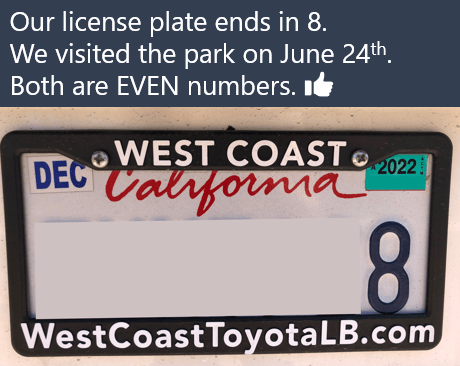
What if your personalized plate doesn't end in a number? Then entry is determined by the last numerical digit found in your plate, wherever that may land.
What if you don't have any digits on your plate at all? Then you get to enter on an odd date. Here are the official park rules for the Alternating License Plate System:
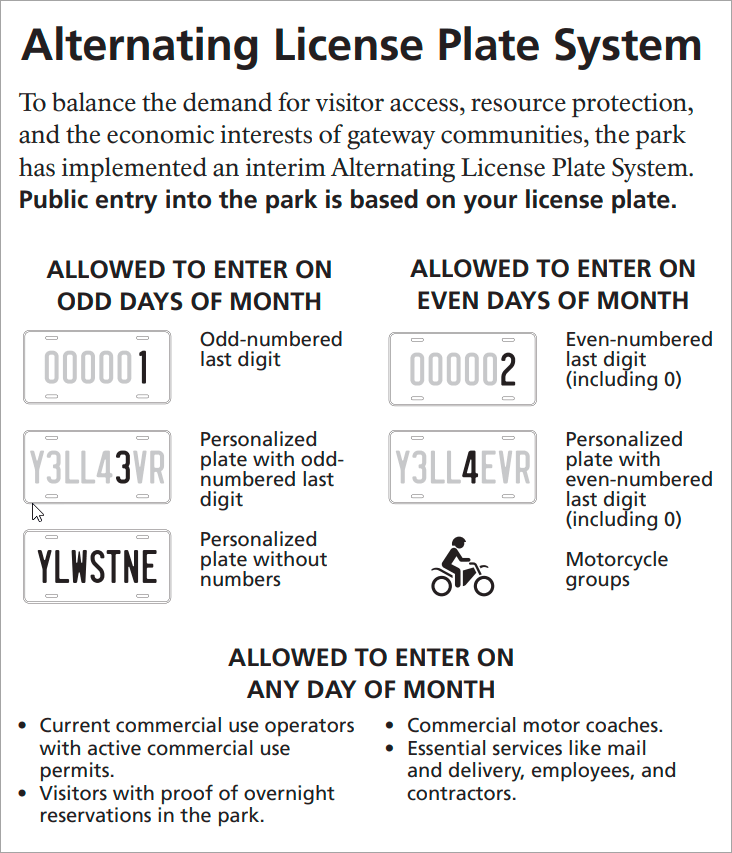
Seeing these rules immediately had me thinking of building a formula in a spreadsheet.
The Challenge
Can you write a formula that assesses a license plate combination and returns the word EVEN or ODD based on the rules above?
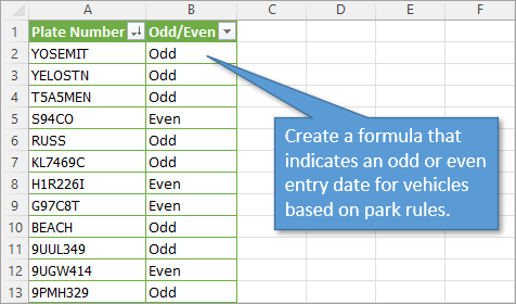
To solve the challenge, just download the Excel file up above and start writing your formula!
Share Your Answer
Please leave a comment on the YouTube video or blog post with your formula solution. I look forward to seeing your solutions and this will be a great learning opportunity for everyone.
Another Way To Solve The Problem
We also found bison out on the road checking plate numbers. They use horns instead of formulas to regulate unwelcome guests… 😬

Similar Posts
If you enjoy challenges like these, you can check out some of the challenges I've posted in the past.
- Baby Shower Guessing Game
- Equal Playing Time
- Seating Chart Planner
- Data Cleansing: Convert Text to Time Values
Conclusion
I'll be back in a few weeks to walk you through possible solutions based on your feedback. Until then, enjoy the challenge!


Yellowstone is such a beautiful area! Enjoy your family trip!
I was able to do it in Excel 2019, but had to use 4 sets of helper cells per plate. So, it’s not pretty, but it works!
Helper #1 – text to columns to break the letters and numbers apart.
Helper #2 – determine if helper #1 is a number and if it is was it even or odd.
Helper #3 – determine if helper #2 was the last digit.
Helper #4 – is the last digit even or odd.
Answer – if statement using helper #4
Consider column B As Helper
In B5 And down I wrote
==ISODD(VALUE(MID([@[Plate Number]],MAX(IF(ISNUMBER(VALUE(MID([@[Plate Number]],ROW(INDIRECT(“1:”&LEN([@[Plate Number]]))),1))),ROW(INDIRECT(“1:”&LEN([@[Plate Number]]))),””)),1)))
Consider column C As Results
In C5 And Down I Wrote
=IFERROR(IF(OR([@[Odd/Even]]=TRUE,ISERR([@[Odd/Even]])),”Odd”,”Even”),”Odd”)
I know it is not an “elegant” solution but it works 🙂
=IFERROR(IF(ISODD(MID([@[Plate Number]];MAX(IF(ISNUMBER(VALUE(MID(A5;ROW(INDIRECT(“1:” & LEN(A5)));1)));ROW(INDIRECT(“1:” & LEN(A5)))));1));”Odd”;”Even”);”Odd”)
=IFERROR(IF(ISODD(MID(C5,MAX(IFERROR(SEARCH({1,2,3,4,5,6,7,8,9,0},C5,SEQUENCE(LEN(C5))),0)),1)),”Odd”,”Even”),”Odd”)
my formula for the license plate challenge is the following formula
=IF(ISEVEN(IFS(ISNUMBER(VALUE(RIGHT(A11,1))),VALUE(RIGHT(A11,1)),ISNUMBER(VALUE(MID(A11,LEN(A11)-1,1))),VALUE(MID(A11,LEN(A11)-1,1)),ISNUMBER(VALUE(MID(A11,LEN(A11)-2,1))),VALUE(MID(A11,LEN(A11)-2,1)),ISNUMBER(VALUE(MID(A11,LEN(A11)-3,1))),VALUE(MID(A11,LEN(A11)-3,1)),ISNUMBER(VALUE(MID(A11,LEN(A11)-4,1))),VALUE(MID(A11,LEN(A11)-4,1)),ISNUMBER(VALUE(MID(A11,LEN(A11)-5,1))),VALUE(MID(A11,LEN(A11)-5,1)),ISNUMBER(VALUE(MID(A11,LEN(A11)-6,1))),VALUE(MID(A11,LEN(A11)-6,1)),TRUE,1)),”Even”,”Odd”)
Pretty long, but functional…
=IF(ISODD(IFNA(RIGHT(LEFT([@[Plate Number]],MATCH(0,INDEX(-MID([@[Plate Number]],ROW(INDIRECT(“1:”&LEN([@[Plate Number]]))),1),0))),1),0)),”Odd”,IF(ISEVEN(IFNA(RIGHT(LEFT([@[Plate Number]],MATCH(0,INDEX(-MID([@[Plate Number]],ROW(INDIRECT(“1:”&LEN([@[Plate Number]]))),1),0))),1),0)),”Even”,IF(IFNA(RIGHT(LEFT([@[Plate Number]],MATCH(0,INDEX(-MID([@[Plate Number]],ROW(INDIRECT(“1:”&LEN([@[Plate Number]]))),1),0))),1),0)=0,”Odd”)))
Jon,
I can offer the following solution.
Start with a helper column (C) with this formula:
=IFERROR(VALUE(RIGHT(IF(SUM(LEN(A5)-LEN(SUBSTITUTE(A5, {“0″,”1″,”2″,”3″,”4″,”5″,”6″,”7″,”8″,”9”}, “”)))>0, SUMPRODUCT(MID(0&A5, LARGE(INDEX(ISNUMBER(–MID(A5,ROW(INDIRECT(“$1:$”&LEN(A5))),1))* ROW(INDIRECT(“$1:$”&LEN(A5))),0), ROW(INDIRECT(“$1:$”&LEN(A5))))+1,1) * 10^ROW(INDIRECT(“$1:$”&LEN(A5)))/10),””),1)),””)
Then in the table use the formula:
=SWITCH(C5,0,”Even”,1,”Odd”,2,”Even”,3,”Odd”,4,”Even”,5,”Odd”,6,”Even”,7,”Odd”,8,”Even”,9,”Odd”,””,”Odd”)
My normal approach would be to use a function which allows for testing and updating in one place.
=IFERROR(IF(MOD(TEXTJOIN(“”,TRUE,IFERROR((MID([@[Plate Number]],ROW(INDIRECT(“1:”&LEN([@[Plate Number]]))),1)*1),””)),2)=0,”Even”,”Odd”),”Odd”)
Jon,
Here is an approach using VBA functions. Use =fPlateDay([@[Plate Number]]) in table.
Public Function fPlateDay(platenumber) As String
‘Determine if car entry is on odd or even days of month
Dim plateno As Variant
plateno = fExtractNumeric(platenumber)
If Len(plateno) > 0 Then
plateno = Right(Val(plateno), 1)
Select Case plateno
Case 0, 2, 4, 6, 8
fPlateDay = “Even”
Case 1, 3, 5, 7, 9
fPlateDay = “Odd”
End Select
Else
fPlateDay = “Odd”
End If
End Function
Public Function fExtractNumeric(strInput) As String
‘ Returns the numeric characters within a string in
‘ sequence in which they are found within the string
Dim strResult As String, strCh As String
Dim intI As Integer
If Not IsNull(strInput) Then
For intI = 1 To Len(strInput)
strCh = Mid(strInput, intI, 1)
Select Case strCh
Case “0” To “9”
strResult = strResult & strCh
Case Else
End Select
Next intI
End If
fExtractNumeric = strResult
End Function
I didn’t quite follow directions – instead of using a formula I created a function, called StringOddEven where the one input argument references the cell containing the license plate number:
Function StringOddEven(MyStr As String) As String
Dim Count As Long
Dim MyChr As String
For Count = Len(MyStr) To 1 Step -1 ‘find first numeric character working back to front
MyChr = Mid(MyStr, Count, 1)
If IsNumeric(MyChr) Then ‘continue if numeric character found
If MyChr Mod 2 = 0 Then
StringOddEven = “EVEN”
Else
StringOddEven = “ODD”
End If
GoTo LExit ‘exit loop: found the furthest right numeric character in input string
Else
End If
Next ‘no numeric characters found so look at next character to left
‘If there are no numeric characters, the result is ODD
StringOddEven = “ODD”
LExit:
End Function
In B5: =IFERROR(IF(ISODD(TAKE(LET(x,MID(A5,SEQUENCE(LEN(A5)),1),FILTER(x,CODE(x)<58)),-1)),"Odd","Even"),"Odd")
(I used standard cell references)
What is the TAKE function?
1. The place of the last number in the string of A5 is (confirm with Ctrl-Shift-Enter):
=MATCH(2,1/ISNUMBER(MID(A5,ROW(INDIRECT(“1:&LEN(A5))),1)*1))
2. That number is (confirm with Ctrl-Shift-Enter):
=MID(A5,MATCH(2,1/ISNUMBER(MID(A5,ROW(INDIRECT(“1:”&LEN(A5))),1)*1)),1)
In case of no number, the result is #NA.
3. If that last number is ODD the result must be ODD, else EVEN, but in case of ERROR (= no numbers (#NA)), the result must also be ODD. In this way we arrive at this result (confirm with Ctrl-Shift-Enter):
=IFERROR(IF(ISODD(MID(A5,MATCH(2,1/ISNUMBER(MID(A5,ROW(INDIRECT(“1:”&LEN(A5))), 1)*1)),1)),”Odd”,”EVEN”),”ODD”)
—————-
My VBA-Solution:
Sub Odd_or_Even()
Dim a As Integer, L As Integer, LR As Integer
Dim t, x As Integer, y As Integer
With Sheets(“Challenge”)
LR = .Cells(.Rows.Count, 1).End(xlUp).Row
For x = 5 To LR
L = Len(.Cells(x, 1))
For y = L To 1 Step -1
a = 0
t = Mid(.Cells(x, 1), y, 1)
If t >= 0 And t <= 9 Then
a = 1
If WorksheetFunction.IsOdd(t) = True Then
.Cells(x, 2).Value = "Odd"
Else
.Cells(x, 2).Value = "Even"
Exit For
End If
Exit For
End If
Next y
If a = 0 Then
.Cells(x, 2).Value = "Odd"
End If
Next x
End With
End Sub
=LET(length,LEN($A5),splitchar,
MID($A5,SEQUENCE(1,length,1,1),1),
transformtovalue,
VALUE(splitchar),
countchar,COUNT(transformtovalue),
lastdigit,RIGHT($A5,1),
lastcharpos,XMATCH(TRUE,ISNUMBER(transformtovalue),0,-1),
lastchar,MID(A5,lastcharpos,1),
IFS(countchar=0,”odd”,ISNUMBER(lastdigit),IFS(ISEVEN(lastdigit),”even”,ISODD(lastdigit),”odd”),ISTEXT(lastdigit),IFS(ISEVEN(lastchar),”even”,ISODD(lastchar),”odd”)))
Perfect scenario for a recursive super simple lambda EO (Even/Odd function), in B5:
=EO([@[Plate Number]])
where EO(A)=
=LAMBDA(a,
LET(
n, LEN(a),
x, –RIGHT(a, 1),
IF(n = 0, “Odd”, IF(ISERR(x), EO(LEFT(a, n – 1)), IF(ISODD(x), “Odd”, “Even”)))
)
)
In my first post, under point 1, a quote (“) is missing. That formula must be:
=MATCH(2,1/ISNUMBER(MID(A5,ROW(INDIRECT(“1:”&LEN(A5))),1)*1))
The solution (first post under 3) should not be changed.
Cool challenge. Thanks Jon.
My solution:
=LET(plate,[@[Plate Number]],
length,LEN(plate),
chars,MID(plate,SEQUENCE(,length,length,-1),1),
nums,FILTER(chars,ISNUMBER(VALUE(chars)),”Odd”),
first_num,INDEX(nums,1),
IFS(first_num=”Odd”,”Odd”,ISODD(first_num),”Odd”,ISEVEN(first_num),”Even”))
Good challenge; thank you.
I used MID, right, isnumber, Value and nested if … I got it right but a little messy with the nested if.
Hi,
my solution (and I can see Renier Wessels came up with very similar):
=LET(
plate, [@[Plate Number]],
plateChars, MID(plate,SEQUENCE(1,LEN(plate)),1),
plateNumsAndErrors, VALUE(plateChars),
plateNums, FILTER(plateNumsAndErrors, ISNUMBER(plateNumsAndErrors)),
numbersCount, COUNT(plateNums),
lastNumber, INDEX(plateNums,1,numbersCount),
IFS(LEN(plate) = 0, “INVALID”, numbersCount = 0, “odd”, ISODD(lastNumber), “odd”, ISEVEN(lastNumber), “even”, TRUE, “—“))
Thanks Jon. This was quite the challenge for me. My solution is:
=IF(ISEVEN(IF(TEXTJOIN(“”,TRUE,IFERROR(–MID(A5,ROW(INDIRECT(“1:”&LEN(A5))),1),””))=””,1,TEXTJOIN(“”,TRUE,IFERROR(–MID(A5,ROW(INDIRECT(“1:”&LEN(A5))),1),””))))=FALSE,”ODD”,”EVEN”)
This gave an otherwise dreary night shift a bit of a boost.
Great challenge Jon! Enjoy your time in the park!
=LET(str,–MID(A5,SEQUENCE(,LEN(A5)),1),
IF(IFERROR(ISODD(XLOOKUP(TRUE,ISNUMBER(str),str,,,-1)),TRUE),”ODD”,”EVEN”))
=IFERROR(IF(MOD(MID([@[Plate Number]];VALUE(MAX(IFERROR(FIND({1,2,3,4,5,6,7,8,9,0};A5;ROW(INDIRECT(“1:”&LEN(A5))));0)));1)/2;1);”Odd”;”Even”);”Odd”)
I love this.
First use SEQUENCE and MID to generate an array of the letters. Then check for values, match TRUE against them in descending order, and use MID to return that letter. Then it’s a simple IF
=IFERROR(IF(ISODD(MID(A1,MATCH(TRUE,LET(n,SEQUENCE (LEN(A1)),NOT(ISERROR(VALUE(MID(A1,n,1))))),1),1)),”Odd”,”Even”),”Odd”)
=IFERROR(IF(ISODD(XLOOKUP(TRUE,ISNUMBER(MID([@[Plate Number]],ROW(INDIRECT(“1:”&LEN([@[Plate Number]]))),1)+0),MID([@[Plate Number]],ROW(INDIRECT(“1:”&LEN([@[Plate Number]]))),1)+0,,0,-1)),”Odd”,”Even”),”Odd”)
For all versions of excel (if 365 or 2021 – ENTER otherwise CTRL+SHIFT+ENTER)
=IF(IFERROR(LOOKUP(2,MOD(–MID(A2,ROW($1:$10),1),2)),1),”Odd”,”Even”)
f we allow a plate number longer than 10 characters, then the reference $1:$10 should be changed to any larger (i.e. $1:$50)
A shorter version of my previous solution.
=IF(LOOKUP(2,MOD(–MID(1&A2,ROW($1:$10),1),2)),”Odd”,”Even”)
=LET(num, CODE(MID(UPPER(tblChallenge[@[Plate Number]]),SEQUENCE(,LEN(tblChallenge[@[Plate Number]]),1,1),1)),
onlynum,FILTER(num,num<65,1),
IF(ISEVEN(INDEX(onlynum,1,COUNT(onlynum))),"Even","Odd"))
I split the plate into an array then filter out all the letters, then I just check if the last character in the remaining array is Even, if it is not it means it is Odd or it would be odd due to empty array on the filter if there were no numbers.
Usng new functionality for simplicity: use TEXTJOIN to get only numbers from a plate of any length by using SEQUENCE, take the MOD of dividing by 2 (setting to 1 if there are no numbers). 0=Even, 1 =Odd.
=SWITCH(IFERROR(MOD(TEXTJOIN(“”, TRUE, IFERROR(MID([@[Plate Number]], SEQUENCE(LEN([@[Plate Number]])), 1) *1, “”)),2),1),0,”Even”,1,”Odd”)
Recursive lambda inside a LET() using fixed-point combinators.
=LET(
p,[@[Plate Number]],
x,LEN(p),
r,LAMBDA(G,x,p,IF(x=0,1,IF(ISNUMBER(VALUE(MID(p,x,1))),MID(p,x,1),G(G,x-1,p)))),
IF(ISODD(r(r,x,p)),”Odd”,”Even”)
)
Used a brute force approach (lots of helper columns). I’m sure there is a more elegant solution. but the logic here is very easy to follow.
Description of my solution:
First I split the License Plate into columns of 1 character:
MID(tblChallenge[@[Plate Number]], SEQUENCE(1,LEN(tblChallenge[@[Plate Number]])), 1)
Next, I use XMATCH to look up a list of numbers 0 – 9 in the spilled array, starting from the end.
Add Zero to convert a “text number” to an actual number:
XMATCH({0,1,2,3,4,5,6,7,8,9},O5#+0,0,-1)
If there is no number in the License Plate, this will give an error.
Used IFERROR to return 0 in this case.
IFERROR(XMATCH({0,1,2,3,4,5,6,7,8,9},O5#+0,0,-1),0)
Then wrap this formula in a MAX formula, to return the highest column number, that
contains a number.
MAX(IFERROR(XMATCH({0,1,2,3,4,5,6,7,8,9},O5#+0,0,-1),0))
This is the formula in column L, and now I now in which position the last number is.
0 is returned, if no number is found.
In column M, I then use Index to return the number from the column that we just found above.
INDEX(O5#,,L5)
I then wrap this in ISEVEN to see, if the number is even or not.
ISEVEN(INDEX(O5#,,L5))
And now an IF Formula. If the number is even, then return “Even”, otherwise return “Odd”.
IF(ISEVEN(INDEX(O5#,,L5)+0)=TRUE,”Even”,”Odd”)
Almost there! :-), Now, in column B another IF formula. If there is no number in the plate,
then Col L contains 0. Then return “Odd”, otherwise return the Even/Odd answer from above.
IF(L5=0,”Odd”,M5)
=IFERROR(IF(ISODD(MID(A5,MAX(IFERROR(FIND({1,2,3,4,5,6,7,8,9,0},A5,ROW(INDIRECT(“1:”&LEN(A5)))),0)),1)),”ODD”,”EVEN”),”Odd”)
To address this specific challenge in my own way, I created one macro to copy license plates from the ‘license plate generator’ tab to the ‘challenge’ tab and then used the Data ‘text to column’ to separate the digits of the license plate. To run the macro, I created nd use the short cut CTRL r
Next, I added another column to the table with a formula to find the last digit in the license plate number.
=IFERROR(INDEX(D5:I5,MATCH(9.99999999999999E+307,D5:I5)),” “)
Lastly, in column B, I used this formula to determine the plate to be eligible on an ODD day or an EVEN day
=IFERROR(IF((ISODD(J5))=TRUE,”ODD”,”EVEN”),”ODD”)
With what I have done, the table size in now A4 to J54.
Works great.
=IFNA(IF(ISEVEN(MID([@[Plate Number]],XMATCH(1,–ISNUMBER(VALUE(MID([@[Plate Number]],SEQUENCE(LEN([@[Plate Number]])),1))),,-1),1)),”Even”,”Odd”),”Odd”)
Formula uses MID and SEQUENCE to isolate each character of the plate and then attempts to convert each character into a VALUE with ISNUMBER to determine if it worked. XMATCH searches last-to-first to find the last instance of a successful numeric conversion, and MID grabs the character from that position, which is then assessed by ISEVEN with IF for an Even or Odd outcome. If no number was found, then the result is #N/A and is handled by IFNA to force an Odd answer.
bulky and notvery elegant, but works
=IFERROR(IF(ISODD(VALUE(MID([@[Plate Number]];LEN([@[Plate Number]])+1-MATCH(TRUE;ISNUMBER(VALUE(MID([@[Plate Number]];SEQUENCE(LEN([@[Plate Number]]);1;LEN([@[Plate Number]]);-1);1)));0);1)));”Odd”;”Even”);”Odd”)
sequence creates a reversed matrix of true/false for numeric characters in the string, match returns the position of the first true value, isodd/mid nested in if/iferror return the odd/even result
Great challenge. I used it as an opportunity to try my first recursive Lambda, which went something like:
=LAMBDA(LPlate,
IF(len(Lplate)>0, ‘check if recursion eliminated all characters
IF(ISNUMBER(VALUE(RIGHT(LPlate,1))), ‘check if rightmost character is numeric
IF(ISEVEN(RIGHT(LPlate,1)),”Even”, ‘check if its even
IF(ISODD(RIGHT(LPlate,1)),”Odd”)), ‘check if its odd
RemoveRightmost(LEFT(LPlate,LEN(LPlate)-1))), ‘remove last character ready for recursion
“Odd”)) ‘ if looped through all characters and no numbers found, return “Odd”
Just needs =RemoveRightmost([@[Plate Number]]) in the Odd/Even column once Lambda is set up in name manager.
Probably a sledgehammer to crack a nut, but I had fun learning a new function!
Thanks
For XL365 or XL2021 (or later)…
=IF(ISODD(LOOKUP(10,0+MID(1&A1,ROW($1:$9),1))),”Odd”,”Even”)
For any version of Excel…
=IF(ISODD(LOOKUP(10,0+MID(1&A1,ROW($1:$9),1))),”Odd”,”Even”)
=IF(IFERROR(ISODD(EXTRACTNUMBERS(A4)),TRUE),”Odd”,”Even”)
Some old mixed with some new.
=IF(ISEVEN(IFERROR(LOOKUP(99^99;–MID([@[Plate Number]];SEQUENCE(LEN([@[Plate Number]]));1));-1));”Even”;”Odd”)
Though actually the if is not required. TRUE/FALSE would be enough for me.
Power Query (disappointedly complex)
let
Source = Excel.CurrentWorkbook(){[Name=”tblChallenge”]}[Content],
IsEven = Table.AddColumn(Source, “Iseven”, each try Number.IsEven(List.Last(List.RemoveNulls(List.Transform(Text.ToList([Plate Number]), each try Number.FromText(_) otherwise null)))) otherwise false, Logical.Type)
in
IsEven
Came up with some shorter stuff
Fx:
= IF(ISEVEN(IFERROR(LOOKUP(10; –MID([@[Plate Number]];SEQUENCE(10);1));-1));”Even”;”Odd”)
PQ:
= List.ReplaceMatchingItems({try Number.IsEven(Number.From(Text.Select([Plate Number], {“0”..”9″}))) otherwise null}, {{true, “even”}, {false, “odd”}}){0}
Wrote solution in VBA. Added date and in column D added license plates that can enter the park on that date.
Sub LicenseOddEven()
Dim License As String
Dim i As Integer
Dim j As Integer
Dim LastRow As Integer
Dim LastNum As Integer
Dim k As Integer
Dim StrLen As Integer
Dim TheDay As Integer
LastRow = Range(“A5”).End(xlDown).Row
LastNum = 0
TheDay = (Day(Date)) Mod 2
cells(2, 2).ClearContents
cells(2, 2).Value = Date
cells(2, 2).NumberFormat = “mm/dd/yyyy”
For k = 5 To LastRow
cells(k, 2).ClearContents
cells(k, 4).ClearContents
Next k
For j = 5 To LastRow
License = cells(j, 1).Value
For i = 1 To Len(License)
If IsNumeric(Mid(License, i, 1)) Then
LastNum = Mid(License, i, 1)
End If
Next i
‘MsgBox (License & ” ” & LastNum)
If LastNum = 0 Then
cells(j, 2).Value = “Odd”
ElseIf LastNum Mod 2 Then
cells(j, 2).Value = “Odd”
Else
cells(j, 2).Value = “Even”
End If
LastNum = 0
Next j
i = 5
For k = 5 To LastRow
If TheDay = 0 And cells(k, 2).Value = “Even” Then
cells(i, 4).Value = cells(k, 1).Value
i = i + 1
End If
If TheDay = 1 And cells(k, 2).Value = “Odd” Then
cells(i, 4).Value = cells(k, 1).Value
i = i + 1
End If
Next k
End Sub
I have ASAP Utilities, which may be cheating, but I applied ASAPEXTRACTNUMBERS() to @[Plate Number], which pulls out integers in the same order they appear in the plate.
Formula =IFERROR(IF(ISEVEN(RIGHT(ASAPEXTRACTNUMBERS([@[Plate Number]]),1))=TRUE,”EVEN”,”ODD”),”Odd”)
Hello,
It was a great challenge! I did it with the following VBA code:
Option Explicit
Sub odd_or_even()
Dim plate_number As String
Dim checked_sign As Variant
Dim sign_position As Long
Dim row_number As Long
For row_number = 5 To 54
plate_number = Cells(row_number, 1).Value
sign_position = Len(plate_number)
For sign_position = Len(plate_number) To 1 Step -1
checked_sign = Mid(plate_number, sign_position, 1)
If IsNumeric(checked_sign) = True Then
If checked_sign Mod 2 = 0 Then
Cells(row_number, 2).Value = “EVEN”
Else
Cells(row_number, 2).Value = “ODD”
End If
Exit For
Else
End If
Cells(row_number, 2).Value = “ODD”
Next sign_position
Next row_number
End Sub
Steps for each Plate Number (PN) in column A:
1 Find number of characters. =LEN($A5)
2 Set column D-J containing (PN) splitted into individual characters arranged in reverse order.
Typical formula =MID($A5,LEN($A5)-COLUMN(B2)+2,1)
3 Set column K-Q with each item corresponding to the number type of the item in
The type is : ODD, EVEN, TEXT
Typical formula =IF(ISNUMBER(VALUE(D5)),IF(ISEVEN(VALUE(D5)),”EVEN”,”ODD”),”TEXT”)
4 Within , use MATCH to find the first position of “ODD” and “EVEN”.
Then convert the position to be referred from the left-end of (PN), ie position of the last digit,
and put the position value in column R with heading ‘odd-last’ or column S with heading ‘even-last’.
In case of error (no odd or even number), “TEXT” is entered.
Typical formula =IFERROR(LEN(A5) – MATCH(“ODD”,K5:Q5,0)+1, “TEXT”)
5 By comparison of the cell centents under ‘odd-last’ and ‘even-last’ using IF function in column B,
=IF(AND(R5=”TEXT”,S5=”TEXT”),”Odd”,
IF(AND(ISNUMBER(R5),ISNUMBER(S5)),IF(R5>S5,”Odd”,”Even”),IF(R5=”TEXT”,”Even”,”Odd”)))
the final result “Odd” or “Even” is obtained.
Further to my comment yesterday, the problem can be solved using named formulas instead of
helper columns D to S as follows:
str_org =$A5
n_char =LEN(str_org)
seq2_8 ={2,3,4,5,6,7,8}
ind_char =MID(str_org,n_char-seq2_8+2,1)
odd_or_even =IF(ISNUMBER(VALUE(ind_char)),IF(ISEVEN(VALUE(ind_char)),”EVEN”,”ODD”),”TEXT”)
odd_last =IFERROR(n_char-MATCH(“ODD”,odd_or_even,0)+1,”TEXT”)
even_last =IFERROR(n_char-MATCH(“EVEN”,odd_or_even,0)+1,”TEXT”)
result =IF(AND(odd_last=”TEXT”,even_last=”TEXT”),”Odd”,IF(AND(ISNUMBER(odd_last),ISNUMBER(even_last)),IF(odd_last>even_last,”Odd”,”Even”),IF(odd_last=”TEXT”,”Even”,”Odd”)))
=result to be entered in cell B5
Great challenge, I loved every aspect of it!
In Power Query add a Custom Column with this formula:
= if Number.IsEven(
Number.From(
Text.End( “1”& Text.Select([Plate Number], {“0”..”9″}), 1 )
) )
then “Even”
else “Odd”
Questions and suggestions: https://www.linkedin.com/in/matthiasfriedmann
Late to the party, but here’s my VBA solution
Option Explicit
Function LPlate(strPlate As String)
Dim intAns As Integer
Dim IntStep As Integer
Dim intChr As Integer
intAns = 1
For IntStep = 1 To Len(strPlate)
intChr = Asc(Mid(strPlate, IntStep, 1))
If intChr >= 48 And intChr <= 57 Then intAns = intChr
Next IntStep
LPlate = "Odd"
If intAns Mod 2 = 0 Then LPlate = "Even"
End Function
Late to the party, but here is my VBA code.
Function LPlate(strPlate As String)
Dim intAns As Integer
Dim IntStep As Integer
Dim intChr As Integer
intAns = 1
For IntStep = 1 To Len(strPlate)
intChr = Asc(Mid(strPlate, IntStep, 1))
If intChr >= 48 And intChr <= 57 Then intAns = intChr
Next IntStep
LPlate = "Odd"
If intAns Mod 2 = 0 Then LPlate = "Even"
End Function
Copied Plates to helper, did “text to col” fixed, length 1 markers.
Repeated use of isnumber in repeated nested if statements
=if(isnumber(lastcol),lastcol,if(isnumber(last-1col), last-1col,if(isnumber(last-2col,….,999))))..)
Then used =if(isodd(resultcol),”ODD,”EVEN”)
1. Created a “Numbers only” column:
IFERROR(TEXTJOIN(“”;TRUE;TOROW(MID([@[Plate Number]];SEQUENCE(1;LEN([@[Plate Number]]);1;1);1)*1;2));”1″)
Explanation:
– By combining MID and SEQUENCE, I split each plate into arrays of LEN([@[Plate Number]] elements.
For example: 123ABC –> 1 | 2 | 3 | A | B | C (6 separate columns)
– I multiplied each element of the array by 1 so that I would get #VALUE! error for letters.
– I used TOROW to “trim” the array by eliminating errors and thus leave numbers only.
– Finally I rejoined the array using TEXTJOIN and used IFERROR to avoid #CALC! errors.
2. Created “Odd/Even” column:
SWITCH(MOD(RIGHT([@[Numbers only]];1)*1;2);0;”Even”;”Odd”)
Explanation:
– I isolated the last digit of each element in “Number only” column, and multiplied it by 1.
– I identified even and odd numbers by using MOD of that number divided by 2 (could have used ISODD or ISEVEN functions as well).
– Thanks to the SWITCH function, if MOD(RIGHT([@[Numbers only]];1)*1;2 = 0 it returns “Even”, else it returns “Odd”
Excellent challenge! Can’t wait to challenge myself!