Bottom Line: Take this Excel Challenge to create a solution that calculates the points and the winner for a guessing game.
Skill Level: Intermediate
Watch the Video
Solution Video
I went live on YouTube to walk through the solution and show some great submissions from our community members (that's you). The recording of the session is below.
This should be a great opportunity to learn some new functions and formulas. I covered the IF, ABS, HOUR, ROUNDDOWN, TEXTBEFORE, LEFT, SEARCH, RANK, FILTER, and LET functions. Plus conditional formatting and many other data analysis techniques.
The SOLUTIONS file below contains a table with a list of all submissions file from the community. There is a column with a description of the file and a link to download the file.
Download the Excel File
You'll need this Excel worksheet to complete the challenge:
And here is the solution file that I will use on the YouTube Live training session.
Here is a version of the file that will work on older versions of Excel, if you experience any issues with the file above.
File for Hosts
If you're hosting a baby shower and just need the Excel file to run the game, then the following file is for you. We've prepared a blank file that contains all of the calculations. You just need to enter the participant names, guesses, and actual results. The winner(s) will automatically be calculated.
And here is a Google Sheets version of the file. Go to File > Make a copy to save a version that you can edit and share.
Baby Shower Guessing Game
My wife recently went to a baby shower where they played a game. All of the attendees had to guess what day the baby would arrive, the time of day the baby would be born, and the weight and length of the baby as well.
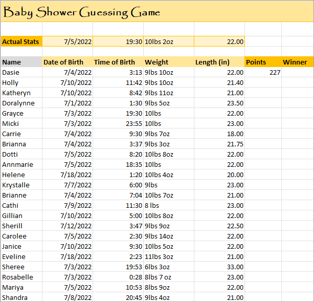
The problem is, they didn't have a practical way to score the guesses, since there are different levels of variance for the four different categories.
I've come up with some scoring rules, but I'd like to have the points tallied automatically based on the actual stats. That's where YOU come in, my friend.
I've entered everyone's guesses into an Excel worksheet and left two blank columns for you to fill as part of an Excel challenge.
The Rules
Here are the rules for scoring each attendee's guesses.
Each participant starts with 50 points per category.
The following points will be deducted from each category when there is a variance between the actual and guessed value.
- Date of Birth: 2 points for each day
- Time of Birth: 1 point for each hour
- Weight: 5 points for each pound (lb)
- Length: 2 points for each inch (in)
Round down to the nearest hour, pound, and inch before calculating the difference for time, weight, and length.
The participant gets 100 points for an exact match in a category. This is the total possible score for the category. They do NOT get 50 + 100. Just 100 points for the category.
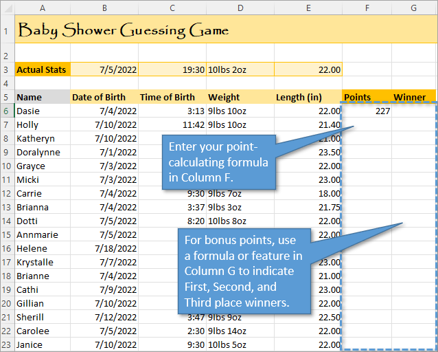
To check your work, you can see the example score in cell F6.
The Challenge
Here's the challenge. I want you to use formulas or other features of Excel to calculate the points for each player and determine who the winner is.
Bonus: Determine who came in second and third place and indicate those placements on the spreadsheet as well.
Upload Your Solution
If you are up to the challenge, we want to see your solution!
Please leave a comment below the post with a brief explanation of how you solved the problem.
You can upload your file with your answers at the link below.
We'll then create a video tutorial with the most popular solutions and explain how to solve the challenge.
Have a question? Leave a comment and we will answer it.
Have fun!


This is fun but the sample points you gave to the first participant had me rather baffled. There’s a 7 hour difference between 19:00 and 3:00 and not 16. The midnight challenge made it much for interesting to me.
Why do you say it’s a 7 hour difference 3:00 is 3 in the morning and 19:00 is 7 in the evening?
I ran into the same issue, but chose to calculate the hour difference WITHIN the calendar day that was chosen. So 19 – 3 is 16. If the date AND time had been combined, the total difference would be totally different.
Correct. When it comes to babies, the time of day and date of birth are two very different talking points. 😉
It states you have to round DOWN – so, 3:00 is 3:00AM of the day of birth – not the following day
(btw, your method would be 8 hrs, not 7)
Yes, You are correct. I calculated the difference in my head before writing the formula. This is why we use Excel.
The variance in hours will only be calculated for the same day. You do not need to go past midnight to calculate the variance between times.
I hope that helps. Thanks! 🙂
I calculate the score for Dasie as 277 not the 227 shown i.e.
Date is 1 day difference – deduct 2 points
Time is 16 hours difference – deduct 16 points
Weight is 1 lb difference – deduct 5 points
Length is correct – no deduction
200 deduct 23 points = 177
Add 100 points for exact length = 277 total
Am I doing something wrong or is the 227 quoted incorrect?
I got the same result (277 vrs.227) so I went back and watched the video again. Nearest I can tell is that an exact match gets 100 points rather than 50, so removing that extra 50 yields the 227.
Count me as the third who was confused. I agree that “100 instead of 50” (as opposed to the original 50 with a 100 bonus) is the only way to match the example answer.
The ‘add 100 points’ (in this case for length) is incorrect: it’s 50 points per category (minus deductions), but 100 if the answer is correct – so, that is a 50 bonus (not 100) – you give her 150 points.
*”The participant gets 100 points for an exact match in a category.”*
48+34+45+100=227
Jay’s explanation is correct. The maximum points for a category is 100 for an exact match. It is not 50 + 100. It’s 50 + 50.
I added some text to the rules on the post to hopefully clarify.
Thanks! 🙂
Hi, You are adding 100 points at the end, instead of 50 🙂 227 is the correct result. You have already considered 50, when calculating the 200 so, you just need to give Dasie the bonus of 50.
weight is not equal, 10lbs vs 9lbs
Oops. I misunderstood the exact match logic. I thought is was AFTER the rounding down. I’m not changing my submission, but I understand it now. 🙂 Thanks, again.
I added four helper columns to build and troubleshoot the formulas to calculate points for each of the four categories. Once the formulas worked I used a LET function in the “Points” column to make the SUM formula more readable. I had a little fun with the “Winner” column using LARGE, SMALL, CHAR functions and conditional formatting.
Wow this is interesting as we do this all the time at work and we do it manually but it seems to be hard and I have no idea how to do it.
The same method used as described by Allen Weber. First 4 helper columns and when it worked transferred to the cell calculating the points with LET.
Hi Jon
For the date of birth answer I used an IFS formula,
for the time of birth answer I used a FLOOR function,
for the weight answer I converted the lb to Oz using CONVERT function, with TEXTBEFORE, TRIM and RIGHT, then added the Oz, rounded it down,
for the length answer used IFS function.
I then created a table with all the data and the answer columns and to find the winner I used a RANK.EQ function ranking the points in order of highest to lowest.
Then created a mini table which tabulated the final positions with their names and the points using INDEX MATCH functions
LOTS OF FUN…the most challenging being the time??? or did I miss an easier way
Interesting challenge. I broke down the task as follows using 5 helper columns.
-Used date math with the absolute function to determine date penalty
-Used hour function with simple math and wrapped result in absolute function for time penalty
-The weight was probably the trickiest as I had to use left and find functions to isolate the number before “lbs”, then wrap it in a value function before doing the match. Finally abs function was used to ignore +/- variances.
-Length required rounding down each value before doing the math and wrapping the result in abs function.
I stored the penalty values in row 3 to facilitate using a different scoring approach.
The points column used 4 nested if statements to add the penalties and bonus points as appropriate.
The rank column (using rank.eq) simply determined everyone’s rank.
Finally, I used a switch statement in the Winner column to identify the winner, runner up, 3rd place winners–otherwise I simply showed their rank.
You could store the base points per category cells H2:K2 and make the scoring a little more dynamic.
Thanks for a distraction from my day job for an hour or so. 🙂
As a parent, I liked the topic, so this is my first entry ever. I hope I did OK. 🙂
In short, I used basic Excel functions I am familiar with:
1. Round down for normalization of values at first.
2. If for exact match, within it else is for calculating score if not exact. Absolute for ensuring there are no issues with negative values.
3. Stats were not a problem. They can be set to the same scale and format with Absolute and Rounddown easily. Except for Weight, where I am using a tad longer formula using Trim, Find and Substitute to get the 2 numeric values extracted. The input table makes it (I suppose on purpose) difficult by not having two columns for pounds and ounces, and randomly adding spaces etc.
I feel I have improved my understanding of UK measurement system. We are used to grams and metres here, but at least I learnt there are 16 ounces in a pound.
And finally, I learnt that, in English, a newborn’s length is taken. Here, we only measure the length of dead people for a coffin! Living are measured for height. 🙂
lol. very nice anecdote!
Very nice challenge!
You have to work very precisely.
I have one question:
What do you want in column G:
a name/names, a number/numbers, or both?
Took the absolute value of the date difference then calculated the date score with an IF statement that set the score – 100 if the dates were equal. Extracted the hour from the times and similarly computed the hour score as the date score. Extracted the pounds by finding the position of the “L” with SEARCH and taking the LEFT characters before the “L”, then computed the score. The length score used the INT to round down and a similar IF to calculate the score. The sum of the scores filled Col F for total points, and the winner(s) selected by using RANK and CHOOSE to print First, Second, and Third places.
I am not familiar with Rank and choose. I going to have to do some research…I look forward to seeing how you used them!
Brandon,
In G6 I used RANK.EQ and CHOOSE this way (column F must be completed):
=IFERROR(CHOOSE(RANK.EQ(F6;F$6:F$28)1,2,3)&”. “&OFFSET(F6,0,-5),””)
I also made a vba-solution in the 2nd sheet of my file, without formulas in the worksheet.
Albert
1. for date i used days function to calculate diff along with abs (to have only positive dates)
2. for time, i used time function to get only hours
3. for weight, i used flashfill
4. for length i used rounddown function
5. for winner, i used rankavg function
I am curious how you used flashfill() and rankavg(). I am not familiar with these.
I look forward to seeing your solution!
Hi Jon, thanks for this fun exercise! I get paid for solving data issues, but honestly it is rewarding on it own.
I have a solution with formulas and with Power Query.
Formulas:
As you get 100 points for exact matches, you need an if condition for each category.
As there are positive and negative deviations, I used ABS for each category.
So basically the calculation is very similar for all categories, with the date being straightforward and some variants for the hours, the pounds and the rounding down. I found the hours the most interesting category and also “rounding down” pounds from a text field is unusual.
As the calculations are so similar, I think it is ok to combine all 4 with plus signs one above the other in one cell. No helper columns or explanations necessary for debugging.
To indicate the First, Second and Third I used Rank.EQ. I think that is best in case of equal points (“Standard Competition Ranking”).
The first 3 ranks are highlighted. The others might be interesting too, so they are visible but a bit greyed out.
For this small task I would normally stick to formulas, but I ❤ Power Query. So here is one way how you can deal with it in Power Query:
I made 2 dynamic ranges for the Actual Stats and the Guesses and queried them From Table/Range.
Changed the data type for each category in both queries.
Brought the Actual Stats to each row of the Guesses.
Similar to the formula description above I combined the four if conditions for each category in one formula.
The annotation is different and the formula have different names, but it is basically the same game as in Excel.
Rebuilding Rank.EQ in Power Query is a bit more complex than in Excel:
-first I added an index to be able to get back to the original order at the end
-sorted descending from highest points to lowest points
-added another order index which is used for the ranking
-grouped the table according to the points, kept all data and added a column with the minimum order value
-expanded the data back
-sorted back to the original order
-got rid of unnecessary columns
=> If you deal with different sources and/or need to automatically update your data then Power Query makes a lot of sense.
=> You can apply the Power Query also in Power BI!
Questions or suggestions: https://www.linkedin.com/in/matthiasfriedmann
Hi Jon, I too, found this a fun challenge. I have Office 2007 so I don’t have access / use of some of the new tools in later versions. I initially thought this was above my current skill level but was happy to find out it wasn’t, and was able to come up with a solution.
My solution just uses a few of the basic formulas and some helper cells (columns). I changed the ‘time’ entries to ‘text’ which made it easier to work with. Changed some of the sheet layout just for aesthetics (row and column size, font, alignment). Also wrote a macro to hide / unhide the points details (helper columns).
Ditto. I used the group method for hiding and unhiding columns & rows. 1 button activation without the macro…lol
Solved with a series of IF functions, converted to a table because they are so handy to propagate formulae and expand as needed for the next baby shower. Could have used LARGE to determine all placements, but went with MAX for first place because it’s shorter.
For column F I used six functions: ABS, HOUR, IF, INT, LEFT, SEARCH, and for column G four: CHOOSE, IFERROR, INDEX, RANK.EQ .
In first instance I thought also to need the function SUBSTITUTE, but on second thoughts I think it’s not necessary.
For column F I used six functions: ABS, HOUR, IF, INT, LEFT, SEARCH, and for column G four: CHOOSE, IFERROR, OFFSET, RANK.EQ .
In first instance I thought also to need the function SUBSTITUTE, but on second thoughts I think it’s not necessary.
I used [=50-(ABS((5-TEXT(B6,”dd”))*2))] to find the raw points for the date of birth. Then [=IF(I6=50,100,I6)] to add the extra 50 points if it was an exact match.
After doing that for each criteria, I entered the points with simple addition [=J6+L6+N6+P6].
From there I used MAX to find the highest value. Then I showed the winner with [=IF(F6=F29,”WINNER”,””)] in column “G”.
Sent to soon.
For the time I used [=50-(ABS(19-HOUR(C6)))], weight [=50-(ABS((10-(SUBSTITUTE(LEFT(D6,2),”l”,””)))*5))], and length [=50-(ABS((22-(ROUNDDOWN(E6,0)))*2))]. I think added the extra 50 points as I did for the date.
Didn’t attempt the bonus. 😉
That’s correct for this shower game, because all dates belong to the same month. To make the formula suitable for other games (with possible dates in different months), it’s better (at my opinion) to abstract DATES instead of DAYS. Example: suppose the date in B6 would be: 6/30/2022, then the result of =ABS(5-TEXT(B6;”dd”)) is 25, where it should be 5. Therefore, I prefer: =ABS(B$3-B6) .
Thank you!
This was the formula I used in the Points column (after naming the Actual Stat cells):
=IF(B6=Birth_Date,100,50-(ABS(B6-Birth_Date)*Date))
+IF(C6=Birth_Time,100,50-(ABS(HOUR(C6)-HOUR(Birth_Time))*Time))
+IF(D6=Birth_Weight,100,50-(ABS(LEFT(D6,FIND(“l”,D6)-1)-LEFT(Birth_Weight,FIND(“l”,Birth_Weight)-1))*Weight))
+IF(E6=Birth_Length,100,50-(ABS(TRUNC(E6)-TRUNC(Birth_Length)*Length)))
Formula for winner:
=IF(F6=LARGE($F$6:$F$28,1),”1st Place”,IF(F6=LARGE($F$6:$F$28,2),”2nd Place”,IF(F6=LARGE($F$6:$F$28,3),”3rd Place”,””)))
Then used conditional formatting to highlight the winner rows
Greetings everyone!
As I have a standalone version of the “non-swoopy” 2016, I tried to keep it as simple and understandable as possible. So anyone with an older version of excel could follow along and still be able to use the formulae.
The result were broken into helper columns to make formulas easier to follow and present data as it is processed. Each of the columns were grouped and hidden for house keeping. One could use this same challenge as a [home]school grade book…;) Instead of “ribbon/medal” placement, it could be used as an order of merit list (OML); based off of a semester grading period. Ask a teacher how they could use it!
First I assessed if each response was an exact match to the real numbers, then I broke each of them down by extracting the info that was relevant. Did some math on the result to arrive at a (-) number. This answer (always -) became the factor multiplied with the point scales of each. The results (-) are then added to the base score for each.
Day: either it is the right day or not. If not, then find the difference. If the difference was positive, then I reversed the math and made it negative.
Time: used hour() to extract the hour as a number…then find the difference. No round down necessary.
Weight: used left(match(“lbs”)) to extract the displayed weight in lbs; converted to a number. Rinse and repeat…no round down required.
Length: essentially the same method as weight…
BONUS:
Used Large() and match() to find 1st, 2nd, and 3rd places.
ADDED BONUS:
Used Vlookup() to to determine and display in a marquis who is in each place
ADDED, ADDED BONUS:
Added a feature for up to 3 TIES in each ranking.
Many cat-skinners here 🙂
Looking fwd to your solution (what is a ‘marquis’?)
Jay, I misspelled it. It’s actually “marquee”.
Movie and live theaters used to have a billboard over the entrance that displayed what was showing or what play was being performed.
Some older theaters still have them. A google search for “apollo marquee” will explain everything. 😉
I know two ‘marquis’: DePompadour and DeSade
And, I think those scrolling (news) tickertapes are also called marquees? I remember in the early webdays, tiny gifs with blinking text were often called that. And then they overdid it with 20 or so on a page!
Anyway, you went fancy – 🙂 https://www.youtube.com/watch?v=KHJHYLKRTi0
Oh…not that fancy. I might have to integrate the scrolling marquee into my next project though…ha ha.
Mine is a simple static display that can change dynamically with the data. Now that I’m thinking about it…a bar graph or shape drawing that displays the winners like the medalists in the Olympics, would be fun too!
Here is a fantastic video on using the helper columns the way I did. He also goes over using array formulas, that are essentially the predecessors of the spill formulas. Where I used Large(), he uses small() with a similar effect.
https://www.youtube.com/watch?v=0PC5ydyQJeo
I originally used Large() to create a random BINGO card generator! It generates 25 cards at a time (originally 70…smh, lol), that can then be printed or copied to another sheet. THEN…as you play the game, you can track the numbers called and it marks ALL of the cards using conditional formatting!
Combined it all into one formula to fill the points column:
=SUM(IF(50-(ABS((B$3-B6)*2))=50,100,(50-(ABS((B$3-B6)*2))))+IF((50-(ABS(19-HOUR(C6)))=50),100,(50-(ABS(19-HOUR(C6)))))+IF(50-(ABS((10-(SUBSTITUTE(LEFT(D6,2),”l”,””)))*5))=50,100,50-(ABS((10-(SUBSTITUTE(LEFT(D6,2),”l”,””)))*5)))+IF(50-(ABS((22-(ROUNDDOWN(E6,0)))*2))=50,100,50-(ABS((22-(ROUNDDOWN(E6,0)))*2))))
Hello – I’d like to add a column for Gender with the rule being that 50 points are awarded if the Gender is guessed correctly. I am having trouble with how to write the formula. The following formula works if the gender (M or F) is correct; however, I get a VALUE error if the gender is guessed incorrectly: =IF(OR(ISBLANK(D5),ISBLANK($X$9)),0,IF(D5=$X$9,50,50+ABS(D5-$X$9)*$T$9)). Can anyone advise?
I think results in your excel it’s wrong, because you have values with 50 in weight, they should be 100 cuz no deductions
Does anyone have this completed spreadsheet they’d be willing to share? I’m no Excel person, nor would I ever be able to complete this exercise. But – there is no excel spreadsheet version available online (that I have found) for my family’s impending baby arrival! All I can offer is my thanks. So – thanks in advance.