Bottom line: Take on this Excel challenge to convert text to time values.
Skill level: Intermediate
Video Explanation
Download the Excel File
You can download the Excel file that contains the data for the challenge below.
The Challenge
This challenge was based on a question from Mark, a member of the Excel Campus community. He exports a report from their training system that contains a column with the total amount of training time that each employee has completed.
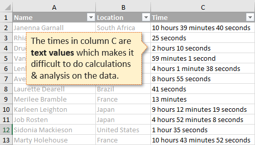
The problem is that the time is a text value written in the following format.
## hour(s) ## minute(s) ## second(s)
The values are NOT recognized by Excel as a date/time data type. This makes it very difficult to do any type of calculations and analysis on the data.
For example, we might want to see a summary report with the average time spent by Location. That will be very easy to create once the data is cleaned up.
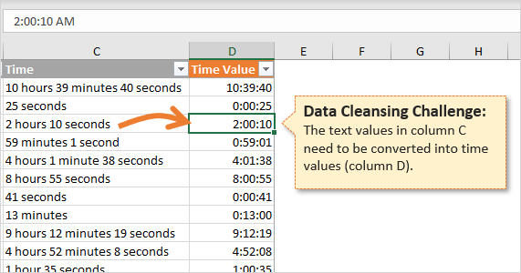
So the challenge is to convert the text values into time values that Excel recognizes.
The Rules
There are only two simple rules for this challenge:
- You can use any Excel tools/features you'd like (formulas, Power Query, VBA, etc.).
- The cells with the results must contain time values. See this article on the Date System in Excel for further explanation.
Share Your Solution
Please leave a comment below (or on the YouTube video) that explains your solution.
You can also upload your solution file to a cloud sharing service (OneDrive, Google Drive, Dropbox) and share the link.
Note: After you leave a comment below you might not see it on the post right away. It takes time to be approved and clear the site cache.
A Great Learning Opportunity
I'm excited to see your solution, and believe this will be a great way for us to all learn from each other.
Here are links to the solution posts where I explain a few popular techniques for converting text to time.
- Convert Text to Time Values with Formulas
- Convert Text to Time Values with Power Query
- Convert Text to Time Values with UDFs in VBA
Thanks again and have a nice day! 🙂


‘=TIME(VALUE(IFERROR(MID(C2,IF(SEARCH(“h”,C2)<5,1,2),2),"0")), VALUE(IFERROR(MID(C2,SEARCH("m",C2)-3,2),"0")),VALUE(IFERROR(MID(C2,SEARCH("sec",C2)-3,2),"0")))
I use the above formula and it works perfectly.
This formula does not correctly handle the 16 instances where the text begins with a single digit number of minutes, but the other formula you posted works for all cases.
=TIME(VALUE(IFERROR(MID(C2,IF(SEARCH(“h”,C2)<5,1,2),2),"0")), VALUE(IFERROR(MID(C2,IF(SEARCH("m",C2)=3,SEARCH("m",C2)-2,SEARCH("m",C2)-3),2),"0")),VALUE(IFERROR(MID(C2,SEARCH("sec",C2)-3,2),"0")))
This work perfectly.
Dear Jon,
I have send you an Excel file with my solution. In the file, I broke down the formula in three parts, extracting the hours, the minutes and the seconds values. The combined formula results in the following:
SOLUTION 1:
=TIME(IFERROR(LEFT(C2,FIND(“hour”,C2)-2),0),RIGHT(IFERROR(LEFT(C2,FIND(“min”,C2)-2),0),2),RIGHT(IFERROR(LEFT(C2,FIND(“sec”,C2)-2),0),2))
SOLUTION 2:
=TIME(IFERROR(LEFT(C2,IFERROR(FIND(“hour”,C2),0)-2),0),IFERROR(MID(C2,IFERROR(FIND(“min”,C2),0)-3,2),0),IFERROR(MID(C2,IFERROR(FIND(“sec”,C2),0)-3,2),0))
It was an interesting challenge, thx Jon
Your first formula works, but your second formula does not correctly handle the 16 instances where the text begins with a single digit number of minutes.
Hi Jon,
Here’s my solution:
=TIME(IFERROR(MID(” “&C2,FIND(“h”,” “&C2)-3,3)+0,0),IFERROR(MID(” “&C2,FIND(“m”,” “&C2)-3,3)+0,0),IFERROR(MID(” “&C2,FIND(“se”,” “&C2)-3,3)+0,0))
Thanks for the challenge!
Cheers,
Kevin Lehrbass
https://www.myspreadsheetlab.com/blog/
I came up with two solutions using VBA. One calculates the time as a fraction of the day, the other uses an array to extract the numbers from the string.
I would note that if you compare the values in your solution to mine, whilst the values shown in the cells are the same there is a small difference in the 15 decimal point…Excel accuracy again!
Graham
Option Explicit
Function ConvertTextToTime1(strText As String) As Double
‘Set target cell to Custom Format hh:mm:ss
Dim intHr As Integer
Dim intMin As Integer
Dim intSec As Integer
Dim intStart As Integer
Dim dblTime As Double
strText = Replace(strText, “s”, “”)
intHr = InStr(strText, “hour”)
intMin = InStr(strText, “minute”)
intSec = InStr(strText, “econd”)
intStart = 1
If intHr > 0 Then
dblTime = Val(Left(strText, intHr – 1)) / 24
intStart = intHr + 5
End If
If intMin > 0 Then
dblTime = dblTime + Val(Mid(strText, intStart, intMin – 1)) / 1440
intStart = intMin + 7
End If
If intSec > 0 Then
dblTime = dblTime + Val(Mid(strText, intStart, intSec – 1)) / 86400
End If
ConvertTextToTime1 = dblTime
End Function
Function ConvertTextToTime2(strText As String) As Double
‘Set target cell to Custom Format hh:mm:ss
Dim arrText() As String
Dim intCount As Integer
Dim strHr As String
Dim strMin As String
Dim strSec As String
arrText = Split(strText)
strHr = “0”
strMin = “0”
strSec = “0”
For intCount = 1 To UBound(arrText) Step 2
Select Case arrText(intCount)
Case “hours”, “hour”
strHr = arrText(intCount – 1)
Case “minutes”, “minute”
strMin = arrText(intCount – 1)
Case “seconds”, “second”
strSec = arrText(intCount – 1)
End Select
Next intCount
ConvertTextToTime2 = TimeValue(strHr & “:” & strMin & “:” & strSec)
End Function
Hi Jon,
I went down the VBA/UDF route as I got quite intimidated by the idea of having to figure out some complex workbook formula.
My main function looks like this:
Function Convert_Text_To_Time(rng As Range) As Single
Dim time_string As String
time_string = rng.Value
Dim transformed_string As String
transformed_string = Substitute_Hours(time_string)
transformed_string = Substitute_Minutes(transformed_string)
transformed_string = Substitute_Seconds(transformed_string)
transformed_string = Remove_Trailing_Plus(transformed_string)
transformed_string = “=” & transformed_string
Dim time_float As Single
time_float = Evaluate(transformed_string)
Convert_Text_To_Time = time_float
End Function
“Helper” functions like Substitute_Hours() are all similar, simple, single-purpose functions that replace part of the original string by appropriate time fractions, for example:
Function Substitute_Hours(input_string As String) As String
‘substitutes word “hour”/”hours” for string “* 1/24 +”
Dim string_to_replace As String
If input_string Like “*hours*” Then
string_to_replace = “hours”
Else
If input_string Like “*hour*” Then
string_to_replace = “hour”
End If
End If
Substitute_Hours = Replace(input_string, string_to_replace, “* 1/24 +”)
End Function
You end up with a decimal number representing the time. For example 0.444213 representing string “10 hours 39 minutes 40 seconds.”
The last step is to set the appropriate time format for the appropriate column.
Thanks for great and challenging challenge. 🙂
Dan
let
Source = Excel.CurrentWorkbook(){[Name=”Table1″]}[Content],
ReplacedValue = Table.ReplaceValue(Source,” hour”,”/24″,Replacer.ReplaceText,{“Time”}),
ReplacedValue1 = Table.ReplaceValue(ReplacedValue,” minute”,”/1440″,Replacer.ReplaceText,{“Time”}),
ReplacedValue2 = Table.ReplaceValue(ReplacedValue1,” second”,”/86400″,Replacer.ReplaceText,{“Time”}),
ReplacedValue3 = Table.ReplaceValue(ReplacedValue2,”s”,””,Replacer.ReplaceText,{“Time”}),
ReplacedValue4 = Table.ReplaceValue(ReplacedValue3,” “,”+”,Replacer.ReplaceText,{“Time”}),
Evaluate = Table.TransformColumns(ReplacedValue4,{{“Time”, each Expression.Evaluate(_,#shared), type text}}),
ChangedType = Table.TransformColumnTypes(Evaluate,{{“Time”, type time}})
in
ChangedType
VBA Solution — first format the answer column as h:mm:ss
then first answer would be =Answer(C1)
Function Answer(rg As Range)
Dim x As String
Dim temp As Long
x = ” ” & rg
hr = InStr(x, “hour”)
mn = InStr(x, “minute”)
sc = InStr(x, “second”)
If hr > 0 Then temp = 3600 * Left(x, 2)
If mn > 0 Then temp = temp + 60 * Mid(x, mn – 3, 3)
If sc > 0 Then temp = temp + Mid(x, sc – 3, 3)
Answer = temp / 60 / 60 / 24
End Function
Looks like I’m a bit late to the picnic, but:
=TIME(IFERROR(LEFT(C2,FIND(“h”,C2)-2),0),IFERROR(MID(C2,MAX(1,FIND(” m”,C2)-2),2),0),IFERROR(MID(C2,MAX(1,FIND(” se”,C2)-2),2),0))
=SUMMPRODUCT(POWER({24,1440,86400},-1);IFERROR(–MID(” “&C2,SEARCH({“hour”,”min”,”sec”},” “&C2)-3,2),0))
my option of function without CSE use
in a formula there can be syntactic mistakes as translated from Russian
That is a very cool and incredibly creative solution! The only tiny problem I see is that the computing of the formula must occasionally accumulate some residual bits because there are 14 instances where Excel thinks the right answer is not the right answer.
Row 979 is an example. The formatted result of this formula is 4:43:23 as expected. However, if you ask Excel if that answer is the same as what is in cell D979, you will get FALSE (no) in response. Even when viewed in decimal format, both times show as 0.196793981. Yet Excel will tell you they are not the same unless your comparison formula includes a ROUND to 9 decimal places.
I know this type of rounding problem is a known, albeit it rare thing with Excel, so I just wanted to point it out for anyone who might be comparing results.
HI,
that was an easy PQ task.: split column, add column with if, merge columns with delimiter :, format as time
let
Source = Excel.Workbook(File.Contents(“\\Mac\Home\Downloads\Text-to-Time-Challenge-Excel-Campus.xlsx”), null, true),
tblExport_Table = Source{[Item=”tblExport”,Kind=”Table”]}[Data],
#”Changed Type” = Table.TransformColumnTypes(tblExport_Table,{{“Name”, type text}, {“Location”, type text}, {“Time”, type text}, {“Time Value”, type datetime}}),
#”Split Column by Delimiter” = Table.SplitColumn(#”Changed Type”, “Time”, Splitter.SplitTextByDelimiter(” “, QuoteStyle.Csv), {“Time.1”, “Time.2”, “Time.3”, “Time.4”, “Time.5”, “Time.6″}),
#”Changed Type1″ = Table.TransformColumnTypes(#”Split Column by Delimiter”,{{“Time.1”, Int64.Type}, {“Time.2”, type text}, {“Time.3”, Int64.Type}, {“Time.4”, type text}, {“Time.5”, Int64.Type}, {“Time.6″, type text}}),
#”Added Custom” = Table.AddColumn(#”Changed Type1″, “Hours”, each if [Time.2] = “hours” then[Time.1] else 0),
#”Added Custom1″ = Table.AddColumn(#”Added Custom”, “Minutes”, each if [Time.2] = “minutes” then [Time.1] else if [Time.4] = “minutes” then [Time.3] else 0),
#”Added Custom2″ = Table.AddColumn(#”Added Custom1″, “Seconds”, each if [Time.2] = “seconds” then [Time.1] else if [Time.4] = “seconds” then [Time.3] else if [Time.6] = “seconds” then[Time.5] else 0),
#”Merged Columns” = Table.CombineColumns(Table.TransformColumnTypes(#”Added Custom2″, {{“Hours”, type text}, {“Minutes”, type text}, {“Seconds”, type text}}, “de-DE”),{“Hours”, “Minutes”, “Seconds”},Combiner.CombineTextByDelimiter(“:”, QuoteStyle.None),”Time”),
#”Changed Type2″ = Table.TransformColumnTypes(#”Merged Columns”,{{“Time”, type time}}),
#”Removed Columns” = Table.RemoveColumns(#”Changed Type2″,{“Time.1”, “Time.2”, “Time.3”, “Time.4”, “Time.5”, “Time.6″}),
#”Changed Type3″ = Table.TransformColumnTypes(#”Removed Columns”,{{“Time Value”, type time}})
in
#”Changed Type3″
My PQ solution was similar to yours:
let
Source = Excel.CurrentWorkbook(){[Name=”Table2″]}[Content],
#”Split Column by Delimiter” = Table.SplitColumn(Source, “Time”, Splitter.SplitTextByDelimiter(” “, QuoteStyle.Csv), {“Time.1”, “Time.2”, “Time.3”, “Time.4”, “Time.5”, “Time.6″}),
#”Added Custom” = Table.AddColumn(#”Split Column by Delimiter”, “hour”, each try if Text.Contains([Time.2], “hour”) then [Time.1] else if Text.Contains([Time.4], “hour”) then [Time.3] else if Text.Contains([Time.6], “hour”) then [Time.5] else 0 otherwise 0),
#”Added Custom1″ = Table.AddColumn(#”Added Custom”, “minute”, each try if Text.Contains([Time.2], “minute”) then [Time.1]
else if Text.Contains([Time.4], “minute”) then [Time.3]
else if Text.Contains([Time.6], “minute”) then [Time.5]
else 0 otherwise 0),
#”Added Custom2″ = Table.AddColumn(#”Added Custom1″, “second”, each try if Text.Contains([Time.2], “second”) then [Time.1]
else if Text.Contains([Time.4], “second”) then [Time.3]
else if Text.Contains([Time.6], “second”) then [Time.5]
else 0 otherwise 0),
#”Merged Columns” = Table.CombineColumns(Table.TransformColumnTypes(#”Added Custom2″, {{“hour”, type text}, {“minute”, type text}, {“second”, type text}}, “en-US”),{“hour”, “minute”, “second”},Combiner.CombineTextByDelimiter(“:”, QuoteStyle.None),”Duration”),
#”Changed Type4″ = Table.TransformColumnTypes(#”Merged Columns”,{{“Duration”, type duration}}),
#”Removed Columns” = Table.RemoveColumns(#”Changed Type4″,{“Time.1”, “Time.2”, “Time.3”, “Time.4”, “Time.5”, “Time.6″})
in
#”Removed Columns”
=TIME(IFERROR(MID(C2,FIND(“h”,C2)>0,2),0),IFERROR(MID(C2,MAX(FIND(“m”,C2)-3,1),2),0),IFERROR(MID(C2,MAX(FIND(“se”,C2)-3,1),2),0))
This formula does the job
=TIJD(+ALS(+NIET(ISFOUT((VIND.ALLES(+LINKS(E$1;1);$C2;1))))=WAAR;+ALS(+VIND.ALLES(” “;$C2)=2;+WAARDE(+DEEL($C2;1;1));+WAARDE(+DEEL($C2;1;2)));0);+ALS(E2=0;+ALS(+NIET(ISFOUT((VIND.ALLES(+LINKS(F$1;1);$C2;1))))=WAAR;+ALS(+VIND.ALLES(” “;$C2)=2;+WAARDE(+DEEL($C2;1;1));+WAARDE(+DEEL($C2;1;2)));0);+ALS(+NIET(ISFOUT((VIND.ALLES(+LINKS(F$1;1);$C2;1))))=WAAR;+ALS(ISFOUT(+WAARDE(+DEEL($C2;9;3)));+ALS(ISFOUT(+WAARDE(+DEEL($C2;8;3)));+WAARDE(+DEEL($C2;7;3));+WAARDE(+DEEL($C2;8;3)));+WAARDE(+DEEL($C2;9;3)));0));+ALS(+NIET(ISFOUT((VIND.ALLES(“con”;$C2))))=WAAR;+WAARDE(+LINKS(+ALS(LINKS(+RECHTS($C2;10);1)=”s”;+RECHTS($C2;9);+RECHTS($C2;10));3));0))
So easy, just use the Autofill function.
1st: Time value is 10 hours 39 minutes 40 seconds. Type 10:39:40 at the right cell
2nd: Time value is 25 seconds. Type 00:00:25 at the right cell
3nd: Click on the right cell of time value and press Ctrl+E and see the result.
in row 22 you know what’s wromg
Tried your method. “2 hours 10 seconds” came out as “2:10:00”. Many more errors.
I’m surprised noone suggested a solution using regular expression. In my opinion that is much more elegant and easier to maintain and modify.
Simply add function and call it in column on the sheet.
Function TextToTime(str As String) As Date
Dim dur As Date
Dim hours As Integer, mins As Integer, seconds As Integer
Dim Matches As Object
Dim re As Object
Set re = CreateObject(“vbscript.regexp”)
re.Pattern = “^(?:(\d+) hours?)? ?(?:(\d+) minutes?)? ?(?:(\d+) seconds?)?$”
Set Matches = re.Execute(str)
hours = CInt(Matches(0).SubMatches(0))
mins = CInt(Matches(0).SubMatches(1))
seconds = CInt(Matches(0).SubMatches(2))
dur = DateAdd(“h”, hours, dur)
dur = DateAdd(“n”, mins, dur)
dur = DateAdd(“s”, seconds, dur)
TextToTime = dur
End Function
I’m trying the UDF on column C, but it’s returning a Value error.
I created “Hour”, Minute, and “Second” Columns, and a fourth column for the result:
=IFERROR(LEFT(C2,FIND(“hour”,C2,1)-2),0)
=IFERROR(MID(C2,FIND(“minute”,C2,1)-3,2),0)
=IFERROR(MID(C2,FIND(“second”,C2,1)-3,2),0)
=TIME([@Hours],[@Minutes],[@Seconds])