Bottom Line: Learn how to create this interactive histogram or distribution chart that displays the details behind the selected chart column. Download the sample file and watch the tutorial video.
Skill level: Intermediate
The Interactive Histogram Chart
Download the File
Get the Details Behind the Columns
Histogram charts are great because they allow you to quickly see how your data is distributed over the entire population.
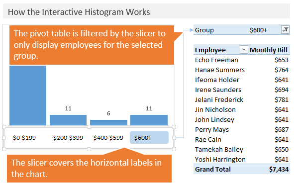
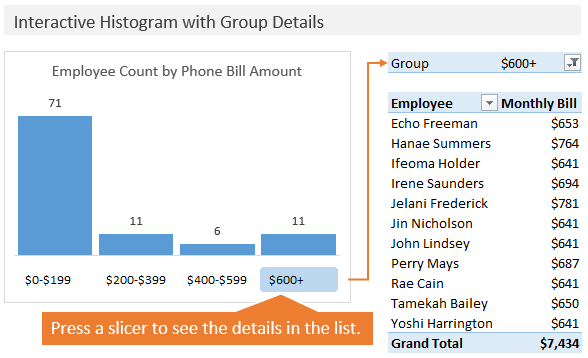
In this example we are looking at data for employees' monthly cell phone bills. The histogram groups the employees by the amount of their individual bill, and then displays the count of the number employees in each group. The chart above shows that there were 71 employees with a monthly cell phone bill between $0 and $199.
It also shows that there were 11 employees with a bill over $600. Whoa! That's a lot time on Facebook! 🙂
So, the first question you might ask is: “Who are the employees with giant bills???”
The pivot table to the right of the chart displays the employee names and their monthly bill amount. It is filtered by a slicer to only display the list of employees for the selected group.
How Does the Chart Work?
The slicer sits on top of the horizontal labels of the chart?. This makes it look like there are labels on the horizontal axis, but it is actually a slicer.
The slicer is connected to the pivot table on the right, and filters by the group name (bill amount range). That pivot table has the Employee Name field in the Rows area and the Sum of the Bill Amount in the Values area.
Checkout the video at the top of the page for detailed instructions on how to create this chart.
The Source Data?
The source data contains one row for each employee with information about the employee and their bill amount. This type of data is usually provided by the cell phone companies.
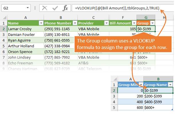
There is a VLOOKUP formula in column G of the Data table that returns the group name. This does a lookup of the Bill Amount to a Group table and returns the Group Name.
You'll notice that the last argument of the vlookup is set to TRUE. This returns the “closest” match for the Bill amount based on the Group Minimum in column A. Checkout my article on VLOOKUP with Closest Match for more details on this technique.?
You can also create the groups automatically with a pivot table, instead of using the VLOOKUP method. However, I like to use the VLOOKUP sometimes because it gives you more control over how you name the group's. You can add custom formatting to the group names, and also control each groups limits.
In this example I am using Excel Tables to store the data and lookup tables. You will also notice that the formulas reference the Tables. This makes the formulas easier to read and write. You don't have to use Tables for this to work, it's just my preferred method.? Checkout my video tutorial on Tables for more details on why they are awesome!
I discuss the pivot table grouping method in this video on pivot tables and dashboards.? I also explain how to create the histogram chart in that video.
The Histogram Pivot Table and Chart
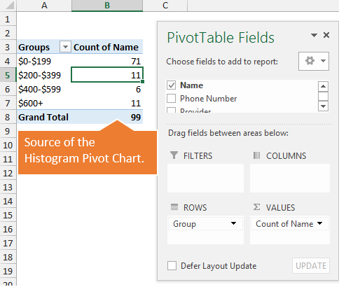
?The image above shows the pivot table that is used to create the histogram chart. The Group name is in the Rows area and the Count of Name is in the Values area. This allows us to plot the distribution of employees on the column chart.
?I explain more about this pivot table in the video at the top of the page.
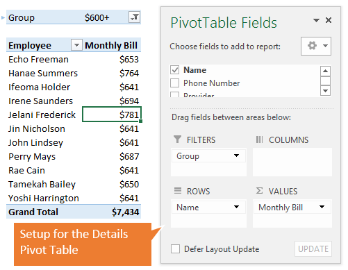
The Details List Pivot Table
The pivot table to the right of the chart displays the details. This pivot table has the:
- Name in the Rows area
- Sum of Bill amount in the Values area
- Group in the Filters area
?The slicer is connected to the pivot table so only the names in the selected group will be displayed. This allows us to quickly see the employees that are included in each group.
Putting It All Together
?Once you have all the components created, it's just a matter of formatting the elements to look good on the page. You can modify the slicer style to give it a cleaner look that will overlay on the chart nicely. I explain more about that in this video on pivot tables and dashboards.
What Else Can We Use This For?
In this example I used data for employee cell phone bills. However, this same technique could be adapted for just about any type of data. Histograms are great because you can quickly see how your data is distributed, but you typically want to dive deeper to see more details about a specific group. You could also add additional fields to the pivot table to view trends or further analyze the subset.
Please leave a comment below with any questions. I'm curious to know what you would use this for? Thanks!
Learn More Dashboard Techniques?
Interested in learning more about dashboards? The following page has links to some great (free) webinars on dashboards.


Frikken BRILLIANT!!!
Thanks Oz!
Sorry, but… The attachment does not open.
Hi Marek,
Are you unable to download the file, or actually open it?
Hi Jon,
I cann’t actually open your file.
Great Trick!
Instead of adding a new column to group, you could use native Pivot Table Grouping. Like here:
http://datapigtechnologies.com/blog/index.php/creating-a-frequency-distribution-with-a-pivot-table/
Thanks Mike! And thanks for the link! I briefly mentioned that in the post and video. The pivot table grouping method is definitely faster. It has a few limits that I always seem to run into, and then default to the lookup table method.
1. The formatting of the text/numbers in the slicer items cannot really be customized with the pivot table groups.
2. The size of the pivot table groups must be the same for each group. That’s probably a rule of histograms anyways, but there’s always the “boss/client pleasing requests” that throw the rule book out the window… 🙂
Either way, it’s good to know both methods and I like your simple explanation. It’s easy to follow. Thanks again!
Hi Jon,
Great technique, thanks for sharing.
Pablo
Thanks Pablo!
Jon,
Great tutorial! Histograms/distribution information can reveal all kinds of “hidden” or not readily-apparent-facts within a data set…everything from determining voter demographics…to what people are really willing to pay for cable/satellite service…and here is a big one:
Say a company has 2 sales people that each sold $200,000 worth of Product “Z” last year. Ok, fine. But what type of buyers are they focusing on?
(I’m just making up numbers here.) A distribution can tell you that salesperson#1 got to $200K via many, many sales in the $500-$1,000 range. Whereas salesperson#2 had significantly fewer sales, but they were mostly in the $2,000 to $5,000 range. Each salesperson has tapped into a different type of buyer – of the same product. That is good information to know.
Thanks for the tutorial.
Hi
Great post inspired me to some new ideas!
One question Is there a good “Count Distinct option in a PivotTable”. I used a count for a KRA so number of people who fell in the range however additional to your example I also integrated a month slicer, if you select multiple months I get the person count twice or however many months you select.
Excellent Job Mr.Jon,
Thank you 🙂
Thanks A!
Very good job JON!
To be perfect you shouldn’t insert the number of column in your lookup formula:
Change the header of table data from “Group” to “Group Name” then find the column number in tblGroups with the MATCH function.
=VLOOKUP([@[Bill Amount]],tblGroups,MATCH(tblData[[#Headers],[Group Name]],tblGroups[#Headers]),TRUE)
Thanks Renato! You are right about using the Match function with Vlookup. You must have read my article on Vlookup & Match. 😉
For quick lookups like this where I know the lookup table is not going to change, I tend to use the hardcoded column number. For a more bullet proof solution I definitely use the Match function. I guess I’m not perfect, but thanks for the tip! 🙂
[…] Read the full article here: Interactive Histogram Chart That Uncovers The Details […]
Jon, thank you for making this so easy to follow. I used it for our donor database when wanting to know the range breakdown for donor giving for the year! It was great!
Very nicely and impressively done. Thanks Jon
Hi Jon and team,
I am running into the following issue when trying to create a Pareto chart. The version I have been using appears as -4111 but when I run the macro it does not like that option:
ActiveSheet.Shapes.AddChart2(201, -4111).Select
I have found the xlPareto but the formatting and details are not as robust as -4111.
ActiveSheet.Shapes.AddChart2(201, xlPareto).Select
Is there a section where this is covered in your course.
Thank you for your time.
Carlos
I am looking to get idea around creating a visual for 3 main fields:
Supplier Name
Due Diligence tasks
Due in Month
I am not able to figure out, how do I combine all 3 in one chart. I can do it 2 separate bar charts but not all together.
Could you please help on this with some example data.