Bottom Line: Learn how the VLOOKUP function works with this simple explanation and example using a Starbucks menu. You can download an example file below to follow along.
Skill Level: Beginner to Expert
In this article you will learn the basic concepts of the VLOOKUP function. I provide a step-by-step guide on how to write a vlookup formula and you can download an Excel file to follow along.
Plus, you will never look at a restaurant menu the same way again… 🙂
Vlookups at Starbucks?
I was standing in line at Starbucks the other day, studying the prices on the menu, and I realized I was doing a bunch of vlookups in my head.
As I scanned down the items on the menu and then looked across to the price columns, I was doing the same thing a vlookup function does.
So I thought this might be a good way to explain the vlookup because everyone can relate to ordering from a food menu. And even if you're already a vlookup expert, this might help you explain the function to your co-workers.
Vlookup Defined
The job of the vlookup is to look for a value (either numbers or text) in a column. Once it finds a match, the vlookup will return a value from any cell in the same row as the match.
The Starbucks Menu Example
Let's look at the Starbucks menu as an example. When looking at the menu I decide that I want to order a Caffe Mocha. I also know that I want a size Grande. Now I need to determine the price to make sure I have enough money to pay for this expensive cup of coffee. 🙂
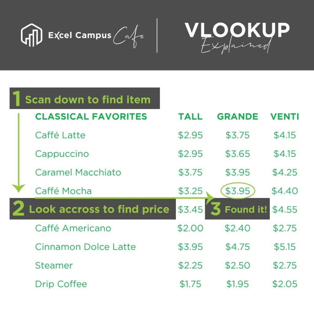
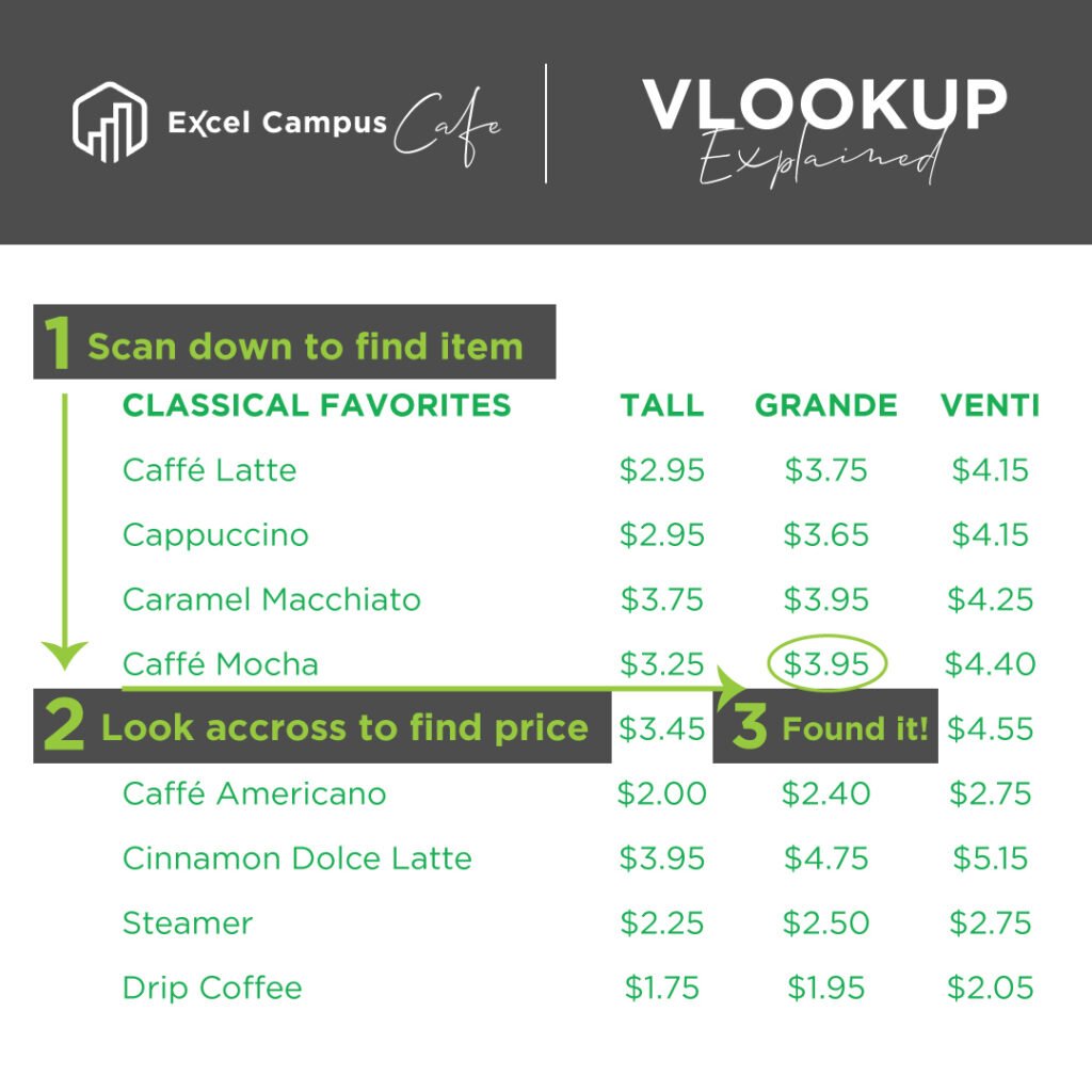
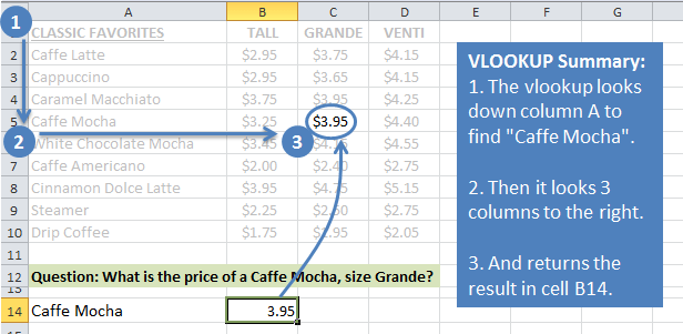
We naturally do this process in a series of steps in our head (see image above):
- First we look down the list of items on the left side of the menu until we find Caffe Mocha.
- Once we find the item, we then look across the columns to the right to find the price.
- The prices for the size Grande items are listed in the 3rd column of the menu, so we scan over to the 3rd column to find our price. There it is, $3.95 for a delicious cup of energy.
Vlookup Example in Excel + Download
Now we'll take a look at how this example works in Excel. I recreated the Starbucks menu in Excel for this example. You can download the file to follow along.
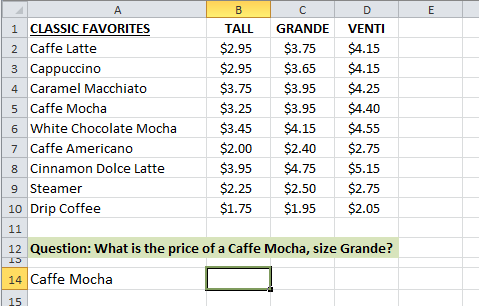
We want to answer the question: “What is the price of a Caffe Mocha, size Grande?”
We will use the vlookup function to answer this question in cell B14.
Vlookup Function Components
First we need to understand the components or arguments that make up the vlookup function. The following image shows the Excel definition of the Vlookup function, and then my simple definition. This simple definition just makes it easier for me to remember the four arguments.
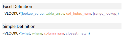
I explain this simple definition below as we walk through an example of creating a vlookup formula.
Creating the Vlookup Formula
Now we will create the vlookup formula to find the price of the Grande Caffe Mocha.
1. lookup_value – This is the what argument.
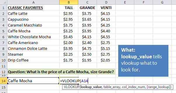
In the first argument we tell the vlookup what we are looking for. In this example we are looking for “Caffe Mocha”. I have entered the text “Caffe Mocha” in cell A14, so we can make a reference to cell A14 in the formula.
We could also add the text “Caffe Mocha” (surrounded in quotes) directly into the formula.
=VLOOKUP(“Caffe Mocha”
But using cell references (A14) makes the formula easier to copy down and reuse for lookups on other items.
2. table_array – This is the where argument.
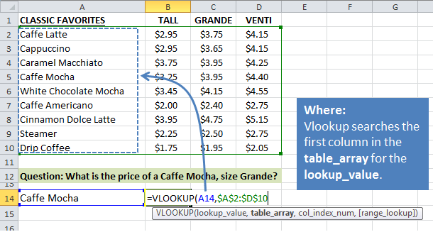
We need to tell the vlookup where to look for “Caffe Mocha”. This argument is specified as a range of cells, and the vlookup will only look in the left column of this range. We also need to include the columns that we want to return a value from. In this case we need to include the price columns because we want to return the price for our lookup_value.
So I reference the range $A$2:$D$10 in the second argument of the function. This means that the vlookup will look through all the rows in column A, from A2 to A10, in search of the value “Caffe Mocha”. Once a match is found it will then look to the right a specific number of columns to return a result.
3. col_index_num – This is the column number argument.
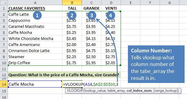
The column number tells the vlookup which column in the table_array we want to return as the result. It counts the columns from left-to-right based on the starting column of the table_array.
Since we want to know the price for the size Grande, I put the number “3” as the third argument of the function. This will return a result from the third column (column C) of the table_array.
4. [range_lookup] – This is the closest match argument.
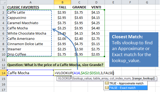
Here we specify whether the vlookup should find an exact match or closest match to the lookup_value. By default, the vlookup will find the closest match to our lookup_value and return a result. This method is best used for looking up numbers.
However, for our example we want to find the exact match to the word “Caffe Mocha”, so I will put “False” for the range_lookup argument. This means that the vlookup will look for an exact match to the value “Caffe Mocha” in the first column of the table_array. If it does not find the word it will return an error (#N/A).
The Result – $3.95 for a Grande Caffe Mocha!
The vlookup formula returns the value 3.95 in cell B14 as expected. This formula can now be reused in other cells to look up other items in the menu. Or you could change the value in cell A14 to a different menu item, “Cappuccino” for example, to instantly see the price for the size Grande Cappuccino.
Conclusion – It's Time for a Coffee!
I hope this helps you understand the basics of how the vlookup function works. Vlookup is one of the most commonly used functions in Excel for looking up data, and it's a great one to know. This article only scratches the surface of what can be done with the vlookup function, but it's best to understand the basics before you learn more advanced techniques.
Most importantly, you now have a good excuse to go out for a coffee break next time you need to explain the vlookup function to a co-worker. 🙂
As always, leave a comment below with any questions or suggestions.
What's Next
This article is part of a series on lookup functions. Please checkout the other articles below.
- VLOOKUP & MATCH – A Dynamic Duo
- The INDEX Function – A Road Map for Your Spreadsheet
- How to Calculate Commissions in Excel with VLOOKUP
- How to Use VLOOKUP to Find the Closest Match – Last Argument is TRUE
Take the VLOOKUP Challenge
I've put together 5-part video training series that will help you learn more about lookup formulas and test your skills.


Jon–Your video of vlookup helped me in transferring data between 3 separate databases, Thank you.
Lmao, why make it so difficult to order a Starbucks xO
Super
Thank you for this explanation!
Amazing! how beautifully and effortlessly explained. I like your videos and post so much that I never want to miss them.
Thank you so much for sharing this post.
I am trying to find duplicate values on two worksheets. In my first attempt I had the worksheet A on the first tab and worksheet B on the second tab. Vlookup gave me all the matched tags.
In my second attempt I reversed the order and had worksheet B on the first tab and worksheet A on the second tab. This time Vlookup gave a different value (lower than the first attempt). Can someone explain why because I was expecting the same result regardless of the worksheet order
Best and clearest explanation on VLOOKUP ever. Now I have a better understanding of VLOOKUP.
I’ve been afraid of this function for years. Thanks for explaining it so it’s easy!