Conditional Formatting for List of Partial Matches

Bottom Line: Learn how to apply conditional formatting to cells that contain a partial match to a list of values.

Skill Level: Intermediate

Watch the Tutorial

Download the Excel File

The Excel file that I use in the video can be downloaded here:

Conditional Formatting for Partial Matches

Let's say you have a list of items and you want to highlight the ones that start with a certain character or series of characters. You can use a formula to search, find, and apply formatting based on a partial match against a list of data.

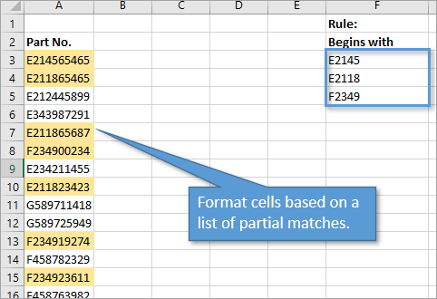
In my example today, I want to color cells for any Part Numbers that begin with a particular list of characters.

Using the Conditional Formatting Window

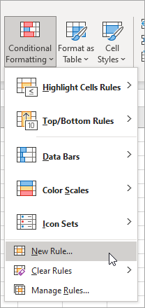
To start, we're going to open up the Conditional Formatting window. You can access this by going to the Home tab on the Ribbon and selecting the Conditional Formatting drop-down menu. Then select New Rule.

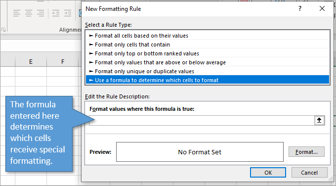
For the Rule Type, choose the option that says Use a formula to determine which cells to format. That will open up a field where you can type or paste a formula. I prefer to write my formulas in a cell and then paste it in, but it's entirely up to you.

Writing the Formula

There are many different lookup formulas and ways to go about this, but we're going to use the COUNTIF function. There are two arguments to COUNTIF. The first is the range, and the second is the criteria.

For range, the formula is looking for the set of data that it should look through to find the criteria. In our case it is our list of 5-character codes that the part numbers should start with. That's F3:F5 on our worksheet. But we want to make those values absolute ($F$3:$F$5) since they won't be changing.

For the criteria, we want to look at the first five characters of the product number. To do that we will use the formula called LEFT. It looks at the leftmost characters up to the number of places you determine. To fill out the arguments for the LEFT function, you choose the first cell in the list (A3) as the text argument, and the number 5 for num_chars argument.

When we close our parenthesis, our complete formula reads:

=COUNTIF($F$3:$F$5,LEFT(A3,5))

When written in the cell, this function returns a value of 1 or 0 depending on if it found those five digits at the beginning of the entry. Any value other than 0 equates to TRUE in the Conditional Formatting window, while a 0 is the same as returning FALSE.

Applying the Formatting

One thing to note is that if you are writing your formula directly into the conditional formatting rule, if you select cell A3 instead of actually typing it, Excel is going to make it an absolute reference ($A$3) by default, which is not what we want.

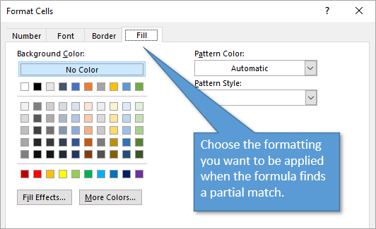
Once the formula is copied or typed into the Conditional Formatting rule, click the Format button. This gives you all of the formatting options you can choose from that will apply when the formula is true.

After hitting OK, the new formatting will appear in the cells where the partial match is true.

If you find that you've accidently applied the rule to the cell where you wrote the formula instead of the list of Part Numbers, you can easily make edits to that range by selecting Manage Rules in the Conditional Formatting drop-down on the Home tab. (That's an edit I often have to make because I forgot to highlight the range I wanted before opening up the rule manager.)

Applying Conditional Formatting to Entire Rows

If you want to expand your conditional formatting so it extends across the entire row, that's easy to do. As mentioned above, you can edit the existing rule by going to the Home tab, clicking the Conditional Formatting drop-down menu, and choosing Manage Rules. From there you can just change the range that the conditional formatting applies to.

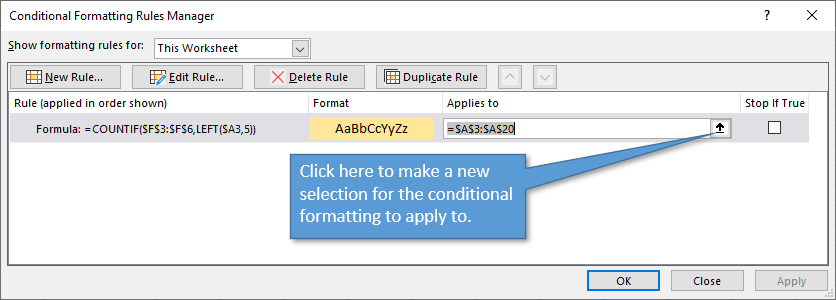
In order for this to work, the column reference in our formula must be absolute ($A3). This is because we want the formatting to be determined based on the values from the original column.

The criteria for the conditional formatting does not have to be on the same sheet as the cells being formatted, and if you want to add, change, or delete some of the criteria for the formatting, just ensure that your formula includes the updated range of cells.

Partial Matches that Aren't at the Beginning

What if the characters you are trying to match fall at the end of the entry instead of the beginning? For example, maybe you want to highlight any entries with the suffix “yahoo.com” in a column of emails. As you can probably guess, you'd simply use the RIGHT function instead of LEFT.

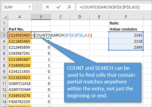
But there may be times when the data you are looking for isn't always in the front or the back of the entry. Or maybe you you're not sure where it would fall because you are not familiar with the entire list of data. For example, maybe you have a list of thousands of inventory product names and you want to call attention to how many contain the description “chocolate” and/or “coffee” anywhere in the name. For this type of partial match, we can use the COUNT and SEARCH functions.

The SEARCH function would look for the entries that contain the words or characters in your list. Then the COUNT function returns a value of 0 if no match is found and 1 (or more) if a match (or more than one match) is found. Here's an image showing how this formula looks.

Conclusion

I hope this helps you to understand how to apply conditional formatting to cells based on partial matches. I've got several other posts that use conditional formatting that I invite you to check out:

• How to Apply Conditional Formatting to Rows Based on Cell Value
• Highlight Rows Between Two Dates with Conditional Formatting in Excel
• How to Filter for Duplicates with Conditional Formatting
• Progress Doughnut Chart with Conditional Formatting in Excel
• How to Apply Conditional Formatting to Pivot Tables

If you have any questions about this process, leave a comment. Thanks for reading!