Bottom Line: Learn how to compare two worksheets for duplicate values by highlighting the cells with conditional formatting. Also highlight values in a different color when there are more than two duplicates.
Skill Level: Intermediate
Watch the Tutorial
Download the Excel File
Here are both the BEFORE and AFTER files from the tutorial.
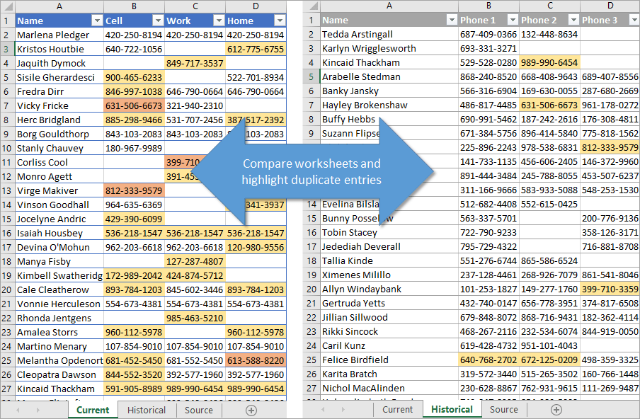
Highlighting Duplicates Between Worksheets
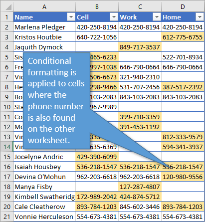
Let's say you have two Excel worksheets that have overlapping data and you want to call attention to any cells that have duplicate entries. You can do so using a formula and conditional formatting.
First let's look at how to write the formula and then we will see how to apply the conditional formatting.
Use the COUNTIF Formula
The formula we'll write is going to examine a cell to see if its contents can be found in another range that we specify. If so, it will return a value of the number of times that data is found. For this process we are using the COUNTIF function.
COUNTIF has two arguments. The first is range and the second is criteria. Range is the group of cells that you want to look in to find a specific value. In my video tutorial, my range is from B2 to F1001 on the “Historical” sheet.
The criteria argument is simply the value that we are looking for. In our example, that's cell B2.
If the value that is found in cell B2 is also found in our designated range on the Historical tab, the COUNTIF function will return a number greater than zero. If it is NOT found on that sheet, it will return a zero.
With conditional formatting, we use those numbers to highlight the entries that are duplicates.
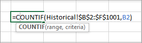
For our example, the formula looks like this:
=COUNTIF(Historical!$B$2:$F$1001,B2)
It's important that the B2 used for the criteria argument is expressed as a relative reference, not an absolute reference. That's because when we apply the conditional formatting to our entire table, Excel will examine each cell individually to see if the criteria apply, but only if it's expressed as a relative reference (no dollar symbols in the reference).
Applying Conditional Formatting
Now that we've looked at how the formula works, let's see how the conditional formatting is applied.
First select the entire range of cells that you want the formatting applied to. In our case it is all of the phone numbers on the “Current” worksheet. On the Home tab of the ribbon, choose the Conditional Formatting drop-down menu and select New Rule.
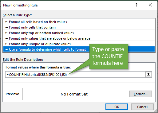
In the New Formatting Rule window, select the option that says Use a formula to determine which cells to format. That will open a field where you can write or paste the formula that we talked about above.
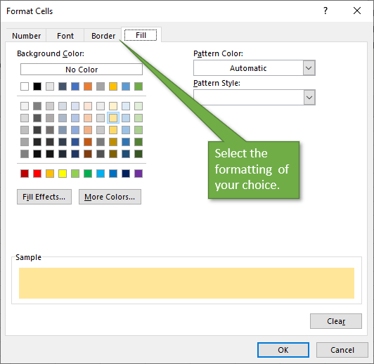
Next, select the Format… button and that will open the Format Cells window, where you can select any type of formatting you wish. Change the font, border, number type, or fill with color so that your duplicates will stand out. When you hit OK, and OK again, your formatting will be applied.
Any cell that returns a value larger than zero will have the new formatting applied.
Different Formatting for Multiple Duplicates
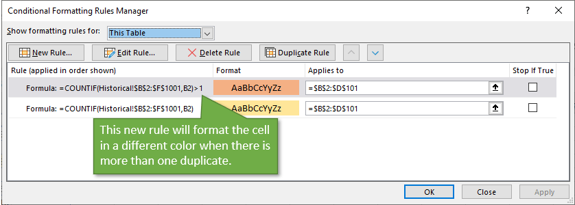
If you'd like to highlight in a different color the entries that have more than one duplicate in the other sheet, you can simply add a new rule.
Start by reopening the Conditional Formatting Rules Manager (Home tab → Conditional Formatting → Manage Rules). We're going to select the rule we've already made and then hit Duplicate Rule. Once the rule is duplicated, select one of them and hit Edit Rule.
The only change we will make to the rule is to add “>1” to the end of the rule. Then we can select Format to choose a different color.
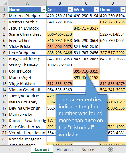
After hitting Apply, we see that our table now shows entries which have more than one duplicate in a different color:
Additional Tutorials
If you'd like to learn more about using conditional formatting, I think you'll find these two posts useful. Check them out:
- Conditional Formatting for List of Partial Matches
- Highlight Rows Between Two Dates with Conditional Formatting in Excel
Conclusion
As you can imagine, there are lots of uses and ways to expand this idea of comparing two sheets and using conditional formatting to highlight those comparisons. If you have any questions or ideas along those lines, I'd love to hear them in the comments below. I hope this was helpful for you.
Have a great day!


Fantastic, thank you.
Great instruction. Would be an added benefit if you could list the phone numbers down a column and return every name that had that number.
Hi Jon! Wonderful information as always! In the particular case of phone numbers, occasionally we see people enter in different formats or even skip the area code. I was wondering if there is a way to use Conditional Formatting to identify cells that do not meet a certain value type (e.g. identify all cells that do not have a ###-###-#### structure). Is that at all possible? Or would you need helper columns in order to do this?
Hi John, I wish to thank you so much for sharing these great skills. Personally, I found this practically helpful.
But I also have one question, I wish to create a data sheet and set a condition where by NO DUPLICATE ENTRIES will be allowed. How do I go about it?
I do not know if you can do that without using an ‘Input Macro’. One issue is if others are using the the database and it just rejects the number it would be very frustrating, they would think they are doing something wrong. The color change, most often, is best as an alert and then you can decide what course of action to take, delete or keep.
Hope this helps.
Hi, Jon, thank you for the tutorial! I used Table references rather than cell references in my COUNTIF statement but the conditional formatting doesn’t seem to accept Table references. Is that true?
Jon made a relevant comment after a blog video from Feb 10th: “I should have mentioned that the Conditional Formatting Manager will not let you reference Tables (structured references) in formulas. However, Diane mentioned a workaround in her comment on creating the named range for the table. Then referencing the named range in the formula.”
Jon, is there a product that will find the duplicate photos saved on a computer. If not, I think you should figure out how to do that, I would buy the product. Thanks
Hi Jon thanks for this I am thinking I could use this to reconcile two sets of data for accounting purposes, anything that was not highlighted was a discrepancy?
I learned about this only recently, this was a nice reminder. I just started a movie database of my collections and this would work well to show which movies have the same actors in them.
As always Jon, you are making me think, thanks for the seeds.
Excellent video. Thanks for the very helpful explanation.
In the window Conditional Rules Formatting Manager on the right there are check boxes to Stop if True. My understanding is that if the box is not checked, after that rule is run, then the next rule is run in order of display. In this case would not all of the orange fills be then replaced with yellow fills since any number not zero would evaluate as true? What am I missing here? Thank you for your help.
Hello I have tried to do the above as its just what I am looking for but got an error message
“You cannot use references to other worksheets or workbooks for Conditional Formatting criteria”…
I keep getting the same error Alison. Did you ever get an answer for this? Also, under Conditional Formatting – Manage Rules, mine does not give me the “Duplicate Rule” option as shown in the video.
Hiya, I admit it this didn’t work straight away, don’t know why?, I did question the version of excel then thought don’t be silly this has to work.
Here is what I did and it has hooray worked yay…
1) Firstly name the tabs so you don’t get confused.
2) Highlight the data and create a defined named range – e.g. right click, name what has worked in the past by using the same name as the tab
3) On your Master sheet (tab) sheet1, highlight the values in column A
4) With the data highlighted, and you have defined the range, you will be able to see the ranges in the top left hand corner to the left of the formula bar.
5) Now Select Format > Conditional Formatting>Use a formula to determine which cells to format.
6) Formula Is: =COUNTIF(Sheet2Data,A1)>0
7) Click on Format… Fill, select any colour.
8) OK > OK – This will now highlight your master copy with any duplicates.
Basically you are;
1) In your Master sheet for the results, but you are
2) Asking conditional formatting to look at your second spreadsheet to check for duplicates.
3) To show duplicates colour them in your Master
spreadsheet
4) Now you can use the filter by colour option and
BOSH! You have your duplicate list. LOVE IT….
I used the Named Range option on both sheets then referred to the name range in the Conditional Formatting.
Hope this helps let me know..
Thank you so much! I was getting the same error and this worked great!
Thanks Jon, this is great .
I have a multi-tab document to track patients across the various stages of their treatment.
I want to use this formula on my master sheet to check for duplicates of the patient reference number across the other sheets, conditionally formatting them to reflect the colour of the tab they are currently in (i.e. duplicate would change to blue if patient was in X-ray but would turn red if they were Discharged) so that patients do not get double booked for appts etc.
I’ve tried to implement this with the help of the above. It works great for my first rule but when I try to add the same formula for the other sheets, it seems to lose reliable function. It appears to randomly format cells which are no duplicates at all.
Can anyone help?
I created all of the conditional formatting on one worksheet which contains the month’s dates, people’s names, a color-coded legend, etc. I want the conditional formatting rules that I created in the first worksheet to be applied to the remaining month worksheets. However, the remaining months don’t match up exactly with the dates from the first month (28, 30, 31 days, weekends fall in different rows, etc.). Also some blocks on the remaining Feb through Dec worksheets already have data in them. I don’t want the cells to be overwritten, just have the rules applied when data is entered in new cells. For example, if someone types ‘Travel’ into the cells corresponding to their name for February 6, 7, 18, 19, 20, I want it to apply the rule that enters Travel with a color-coded grey box with black text. When I do the Format Painter option, it copies from the January worksheet and replaces some of the items already in those February cells. Not what I want. Any suggestions?
This sucked
Losers need to approve comments, cause ur help is garbage
I cannot get this to work completely. I have tab ‘Home’ and tab ‘Away’. ‘Home’ is my sheet I am using as my current tab. I am comparing ‘Home’ to my second tab ‘Away’. I highlight my range and while clicked on ‘Home’, I input my formula: =COUNTIF(Away!$B$2:$D$60,B2)
I get highlighted cells…but they are not values from my second tab. (i.e. It highlights ‘Williams’, but ‘Williams’ ONLY appears on ‘Home’, not on ‘Away’.)
Also, I have values on both tabs that I personally put in and so I know they are identical…this formula doesn’t highlight those values. Very frustrating.
i.e. – I have ‘Matt’ on both tabs . Matt does not highlight. I have the name in two different rows, but that shouldn’t make a difference…it should highlight ‘Matt’ as a duplicate. My columns are in the same order for both sheets.
As I said, very frustrating.
Thank you for this! Does conditional formatting work for multiple sheets, not just one additional sheet?
I posted this in youtube but if ever I get a quicker result here:`
here seems to be a bug with the function which I have been fighting with for some time. at 4:40 we see rows 64 and 65 have been highlighted but the actual function returns 0.
do you have a fix for this?
the process described in the video did not produce the same results. My returned value only came back to one cell, rather than the length of the worksheet. I used the exact formula but it did not seem to work. What step did I miss?
Excelent help, thanks a lot
This is exactly what I needed! Thank you!!
Thank you so much! I’ve been doing it manually this whole time and then I saw your post!
Hello, I want to know if what formula I will use in excel when I wanted to locate a duplicate of an ID Number with different name holder. Hoping that you can help me. Thank You!
How do you make this formatting work if the range is across multiple sheets?
I have 4 sheets within a workbook that I need to check for duplicates. How do I input the range to reflect multiple sheets in the same work book?
Thanks for this, the formula helped me get started with highlighting duplicates in 2 columns on 2 different sheets. A quicker way of duplicating the rule though, is to simply use the Format Painter to copy from the first cell down to the rest and works perfectly.
This video was super helpful and exactly what I needed. Thank you for sharing!
How do you base the duplicates off of a criteria that looks to see if name is the same 1st, then if the same number exists.
This is more of being based off of Dates in my sheets.
Sheet1 : ColA : ColB
1/20/24 : John
2/10/24 : Frank
2/15/24 : John
Sheet2 : ColA : ColB
1/5/24 : John
2/15/24 : Frank
2/15/24 : John
The result that needs to be highlighted is 2/15/24 : John. Because the dates matched AND the name matched.