How to Apply Conditional Formatting to Rows Based on Cell Value

Bottom Line: Learn to change the formatting of an entire row of data based on the value of one of the cells found in that row.

Skill Level: Intermediate

Video Tutorial

Download the Excel File

If you'd like to download the same file that I use in the video so you can see how it works firsthand, here it is:

Format an Entire Row Based on a Cell Value

Sometimes our spreadsheets can be overwhelming to our readers.  Especially when you have a large sheet of data with a lot of rows and columns.  The reader needs to see all the data, but we also want to draw attention to some rows based on a condition.

In this week’s post, I answer a question from Dawna, a member of one of our training programs.  She wanted to highlight the entire rows in a data set when the value in a cell in the row matched a value in a cell outside the table.

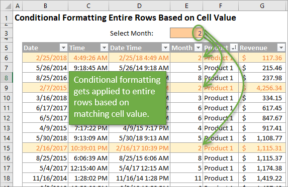
For this scenario, we can use Conditional Formatting.  This is a great feature of Excel that brings life to our spreadsheets and makes them much easier to read.  

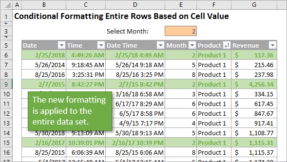
Conditional formatting also makes your files dynamic and interactive.  The user can quickly change the cell that contains the criteria and the matching rows will be highlighted. 

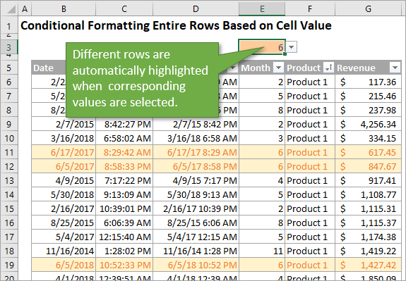
In the image above I changed the value in cell E3 to 6. All rows that contain a 6 in column E are immediately formatted with the font & fill color I specified in the conditional formatting rule.

Conditional formatting is a fun feature that your boss and co-workers will love. Let's get it set up!

Setting Up the Conditional Formatting

The video above walks through these steps in more detail:

1. Start by deciding which column contains the data you want to be the basis of the conditional formatting. In my example, that would be the Month column (Column E).
2. Select the cell in the first row for that column in the table. In my case, that would be E6.
3. On the Home tab of the Ribbon, select the Conditional Formatting drop-down and click on Manage Rules…. That will bring up the Conditional Formatting Rules Manager window.
4. Click on New Rule. This will open the New Formatting Rule window.
5. Under Select a Rule Type, choose Use a formula to determine which cells to format.
6. Under Format values where this formula is true, you are going to write a very simple formula. The formula should set the cell that you want the conditional formatting applied from equal to the first cell in the column that you already identified in Step 1. So in our example the formula would read =$E$3=$E$6.
7. To ensure that the conditional formatting applies to all of the rows in the table, we need to change the absolute relative referencing. In other words, we are going to remove that dollar sign in front of the 6 in our formula. You can either manually delete it, or you can hit F4 twice to accomplish this step.
8. Click on the Format… button to choose whatever format options you like. You can change the font, the fill, the border, etc.

Your New Formatting Rule window should look something like this:

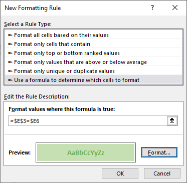
Conditional Formatting Rule

Once you hit OK, you will be taken back to the Conditional Formatting Rules Manager window. Here you will see the rule that you just created.

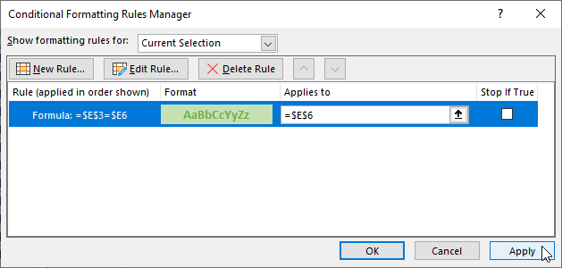
You can click on Apply, but at this point the rule will only be applied to cell E6 because that is the cell you started from and it is what's listed in the Applies to field. We want to extend this rule to the whole table.

To do that, click on the icon to the right of that field (it has an upward facing arrow) and select the range of the entire table. In the example, this would be the data ranging from B6 to G1002 (=$B$6:$G$1002).

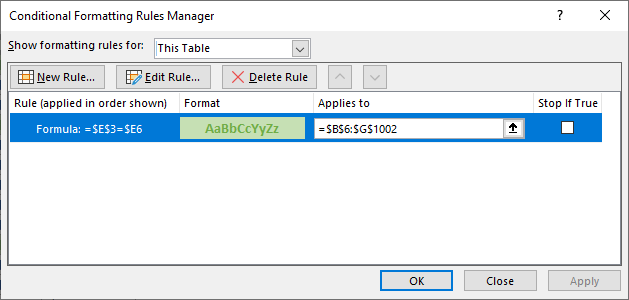
Click Apply one more time and the new formatting applies to the entire data set.

Using Other Comparison Operators

The rule that you create doesn't always have to set a value equal to (=) another value. You can change the format for rows that are

• less than (<),
• less than or equal to (<=),
• greater than (>),
• greater than or equal to (>=),
• or not equal to (<>)

any specific value. And it doesn't have to be a number. It can be text, dates, or other data types as well.

It doesn't matter which of those comparison operators you use. The conditional formatting is just applied based on whether your logic statements are true or false.

If you'd like to get a better understanding of logic statements, as well as IF functions, I recommend this tutorial:

IF Function Explained: How to Write an IF Statement Formula in Excel

The sample file also uses a drop-down list (data validation list) in cell E3. Check out my article on How to Create Drop-down Lists in Cells – Data Validation Lists to learn more.

Conclusion

I hope this is helpful to you. If you have any questions about the process, please leave them in the comments. You can also leave any suggestions or recommendations you might have on the topic.

Thank you!