Bottom Line: Learn how to quickly check if there are values, formulas, or text in a row or column that are different from the other entries.
Skill Level: Beginner
Video Tutorial
Download the Excel File
If you'd like to download the same workbook that I use in the video, you can get it here:
Selecting Cells with Differences
This is a great tip for anyone who is auditing or reviewing a spreadsheet and wants to quickly find any abnormalities in the formulas or values that are being used for calculations.
For example, in the spreadsheet that I use in the video, we want to quickly look for any cells where the sales commission is calculated differently from the norm.
You can easily select cells with differences or variations in formulas or values.
To do that, we start by highlighting the entries in a particular column that we want to check. Then we simply use the keyboard shortcut Ctrl + Shift + \ (backslash).
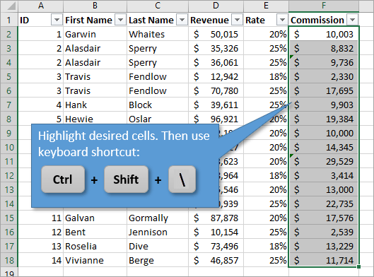
Note: The active cell in your highlighted column will be the basis for comparison. Using the keyboard shortcut will select all the abnormalities based on the formula in that active cell.
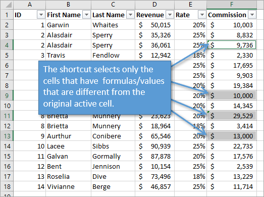
Flag or Highlight the Abnormal Cells
Once all of the cells with differences (exceptions or irregularities) are selected, we can then flag them for review.
With the abnormal cells selected, you can easily change the fill color for those cells, then filter by color to see only those cells. This is especially useful if your data set has a lot of rows.
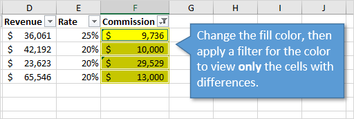
Check out my free 3-part video series on filters to learn more about filtering by color.
You can also add a cell comment/note to flag the differences. Check out the video above for instructions on these techniques.
How to View the Formula Text
Now, looking at the image above, you can't tell that the formulas for those four cells are any different, so let me show you the table with the formulas revealed.
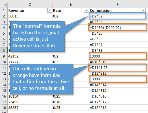
The shortcut to show all of the formulas on a spreadsheet is Ctrl + ~ (tilde). Press it again to toggle back to view the values. You can also press the Show Formulas button on the Formulas tab of the ribbon.
The FORMULATEXT Function
Microsoft introduced the FORMULATEXT function in Excel 2013. The function returns the text of the formula to the cell.
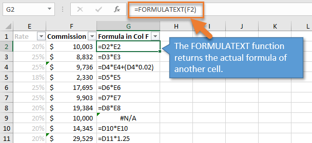
This makes it easy to see both the result of the formulas and the text of the formulas in an adjacent column/row.
You can wrap the function in IFERROR or IFNA to return a different result for cells that do not contain formulas.
=IFNA(FORMULATEXT(F2),"Value")
Using the Go To Special Window
If you're more of a mouse user, you can also select cells with differences in the Go To Special window.
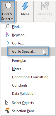
1. From the Home Tab on the Ribbon, choose the Find & Select button. This brings up a drop-down menu.2. Click on Go To Special…
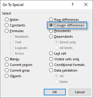
3. This will open up the Go To Special window, where you can select Column differences.
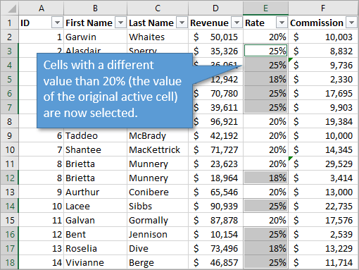
4. When you hit OK, only the cells that have values different from the original active cell will be selected.
It Works for Rows Too
All of the above instructions work for differences in rows instead of columns. The only change is that the keyboard shortcut is Ctrl + \.
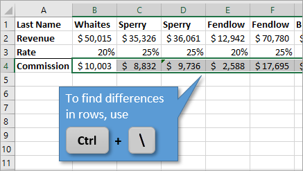
Obviously, when using the Go To Special window, you are going to choose the Row differences option rather than the Column differences.
And as with the columns, you can find differences in values (whether numbers or text), and not just differences in formulas.
Related Post
If you like this keyboard shortcut, check out some of my other favorites in this post: 5 Keyboard Shortcuts for Rows and Columns in Excel.
Conclusion
I hope this tip was helpful, especially if you need to review or audit a spreadsheet for any potential errors in the way it is calculating results. Do you have other tips for auditing workbooks? If so, let us know in the comments below.


Very helpful, thank you.
Thank you, Mark! 🙂
Jon,
I like that you mention the examples of potential use (auditing workbooks).
I find this extremely helpful as sometime I see all those great tips and don’t know how it should be applied to a ‘real world’ problem. I would appreciate more tips that start with a problem and then a solution to solve it.
Thanks for your great work.
Thank you for the suggestion, Natalie! We will definitely do more of this problem > solution explanation in the future. 🙂
Very nice, but unfortunately the shortcut does not seem to work with a french keyboard (I also tried other combinations without success) and incidentally “Go To Special” in the french version is “Select the cells…” (Sélectionner les cellules), that is probably more clear than Go to special, but more difficult to find!
Sorry I first didn’t think of using the Windows key. It works
with Ctrl + Windows + ) for columns and
with Ctrl + Windows + ( for rows.
Awesome! Happy to hear you figured it out and thank you for sharing, Jacsimo! 🙂
As always great information and information that the day by day excel user can use. Much appreciated and looking forward to the next batch.
Sean
Belgium
Thank you, Sean! I appreciate your support! 🙂
Ctrl+Shift+\ (backslash) worked on my system. It did not work with the forward slash as you indicated in your post. This was a great post …… especially as I like to keep ahead of the auditors and am just going into audit season (…. does that make me an auditee?? lol). Great post as always Jon – thanks.
I’m sorry about that. We had a few typos in the original post that have since been corrected.
Yes, you are an auditee (or victim) LOL. Thanks again and have a good one! 🙂
Hi Jon,
Another useful synergy of keyboard shortcuts include Ctrl+[ followed by Ctrl+G>Enter
Real world problem: creating a validation sheet in your workbook based on simple logic test e.g., B12=D12 True or False.
For example, If you used the paste special links option to transfer the same formulas to the validation sheet, and then wanted to navigate quickly between the two sheets. You can use the Ctrl+[ to jump straight back to original place where formula was entered and to get back to your other sheet where you pasted links, simply Ctrl+G>Enter.
Just a quick way to navigate a large workbook with many sheets and repeating formulas.
Thanks,
Colin
Can more than one row or column be audited at a time? When I first read your post it went into the well-that’s-interesting pile. A couple of days later I happened to notice an off-by-one error in an important spreadsheet. Checking revealed that 2 out of 366 formulas in a column had gotten slightly munged.
Now the rest of the columns are suspect. Did columns AA-AN one column at time (No cells were found) but wonder if there is a faster way to audit the remaining columns.
Thank you for the great weekly reading you provide!
Fred
Hi Jon, thanks for these seriously helpful tips. My keyboard has a “back quote” and a “tilde” on the same key and have to press “Shift” first to get a tilde. However, I have noticed that viewing formulae on my laptop is via Ctrl + `
I must say you have really touched the lives of many in the world of excel.
Great post Jon. Very very useful. As always, well explained, well laid out.
Clearly this is an issue, and this is a great solution.
Love your videos.
Christopher