How to Filter for Duplicates with Conditional Formatting

Bottom line: In this video you will learn one technique to quickly filter a column for duplicate values.

Skill level: Beginner

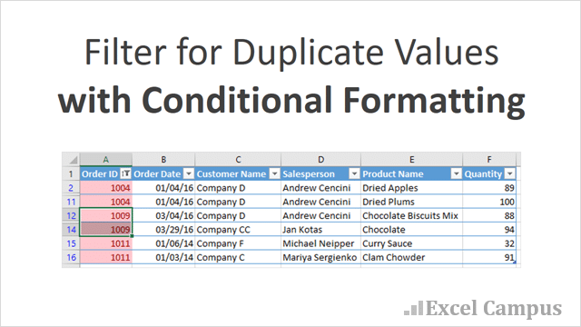
Video: Filter for Duplicates with Conditional Formatting

Double-click video to watch full screen HD.

The video above is a sample from The Filters 101 Course.  This is an online course that covers tips and techniques for filtering to help prepare and analyze your data.

Download Excel File

Download the Excel file to follow along.

Filtering for Duplicates

There are a lot of ways to find duplicates in your data set.  The video above covers one technique using conditional formatting.  This is quick and easy technique to highlight duplicates and apply a filter to only display the rows that contain duplicates.

This technique was suggested by Jen Snyder (a member of the Excel Campus community) on my first video in the 3-part series on Excel Filters.  Thanks again for the great suggestion Jen! 🙂

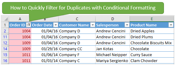
I use an Excel Table in this example, but you do NOT need to use Excel Tables for this to work.  Tables just save a bit of time with this process.  Checkout my video on a Beginner's Guide to Excel Tables to learn more about this awesome tool.

Here are the steps to filter for duplicates with conditional formatting.

Step 1: Apply Conditional Formatting for Duplicates

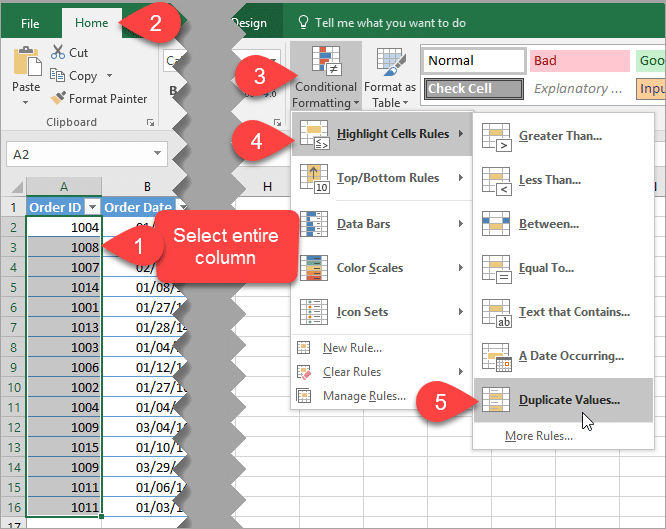
The first step is to select the entire column that you want to find duplicates in.  If you are using an Excel Table then you can select any cell inside the column and press Ctrl+Space Bar.

Ctrl+Space Bar is the keyboard shortcut to select the Entire Column of the Table.

Once the column is selected:

1. Select the entire column.
2. Go to the Home tab of the Ribbon.
3. Open the Conditional Formatting drop-down menu.
4. Select “Highlight Cell Rules”.
5. Then select “Duplicate Values…”
   
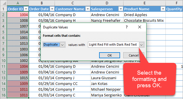
6. That will open the Duplicate Values Window.
7. Choose the formatting you want to apply and click OK.
   

The formatting will be applied to the cells that contain duplicates in the column.

Step 2: Filter the Column for Font or Fill Color

We can now apply a Color Filter to the column.  If you are using an Excel Table then the Filters will already be turned on and you will see the Filter Drop-down Menus in the header row of the Table.

If you are not using a Table then you will need to turn on the Filters for the range.  Checkout my 3-Part video series on Filters to learn how to work with Filters.

To filter for font or fill color:

1. Press the filter drop-down button in the header to open the filter drop-down menu (keyboard shortcut: Alt+Down Arrow).
2. Select “Filter by Color.”
3. Then select the font or fill color that was created by the conditional formatting.  In this example I will choose the red font color because that is the font color applied by the conditional formatting.

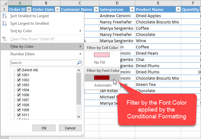
The column has been filtered to only display rows that contain duplicates.

Step 3 (Optional): Group the Duplicate Values with Sorting

The filtered range now shows all the duplicate values.  Those duplicates might be in different rows and look a bit scattered.

We can group the rows together by applying sorting to the column:

1. Press the filter drop-down button in the header to open the filter drop-down menu (keyboard shortcut: Alt+Down Arrow).
2. Pres the “Sort A to Z” or “Sort Smallest to Largest” option to sort the column in ascending order.

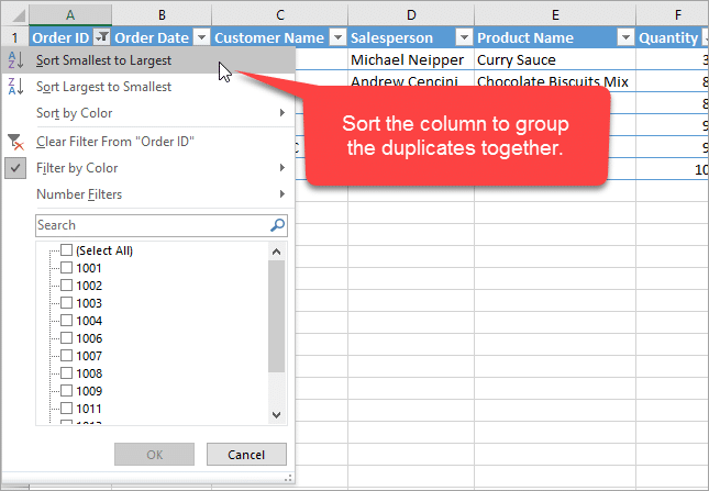
The rows will be sorted and the duplicate values will all appear together.  This makes it easier to look at the duplicates and further analyze them.

Take Action on the Duplicates

Once we have the data range filtered for duplicates, we can then take the next steps to resolve the problem.  This might mean that we need to go to the source of the data, system or person, and determine why duplicates were created.

We also might want to create metrics on the duplicates to use for further analysis.  There are A LOT of reasons to find duplicates in our data sets, and this technique is a very quick way to highlight and filter for the duplicates to see them all in one place.

New Lessons & Bonuses Add to The Filters 101 Course

The video above is a lesson from The Filters 101 Course.  This is one way to filter for duplicates.

There are additional video lessons in the course on how to filter for duplicates using the COUNTIF and COUNTIFS functions.  We can also use these techniques to filter for unique values.

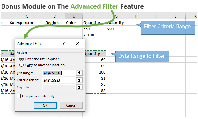
New Bonus Module on Advanced Filter

I have also added a new bonus module to the course on the Advanced Filter.  The Advanced Filter is another tool built into Excel that allows us to apply filters with more advanced and complex logic.  It works well for applying AND & OR logic filters with multiple criteria across multiple columns.

New Bonus Video on Shortcuts for Excel Tables

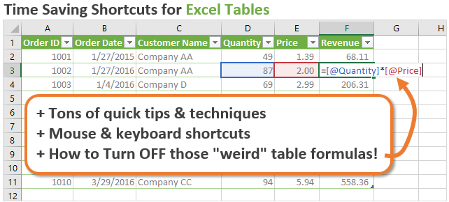
Additionally, I added a bonus video on Shortcuts for Excel Tables.  This includes both mouse and keyboard shortcuts that will save you a lot of time when working with Excel Tables.  If you don't like Tables because of the “weird” formulas, I explain how to turn those formulas off and still benefit from all the great features of Tables.  That entire video is now included with The Filters 101 Course.

Join Filters 101 Before the Discount Expires

The Filters 101 Course is an online course that contains simple step-by-step video tutorials.  It is packed with filtering techniques I have used throughout my career to help me prepare and analyze data faster.

This course, plus my new Filter Mate Add-in will save you a ton of time when working with filters in Excel.

You can currently save over 40% when you buy Filter Mate & Filters 101.  The discount expires this Friday at midnight PST.

Click here to learn more about The Filters 101 Course & The Filter Mate Add-in

Please leave a comment below with any questions.