

As Excel files grow, they get harder to use. More tabs, more data, more chances for someone to type “Miscellaneous” wrong or hunt through a 10-tab workbook just to find the report they need.
In this post, I'm walking through 7 hidden buttons and controls you can add to your spreadsheets right now to make them faster to navigate, easier to update, and a lot more user-friendly. We'll go from simple checkboxes all the way to custom data entry forms.
Download the Excel Files
Complete the form below to instantly access the Excel files.
The xlsm version of the file contains macros and the userform. Macro enabled files have an additional setting you must change when downloaded from the internet.
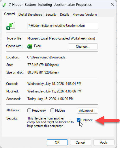
After downloading the file, you will need to Unblock it.
Right-click the file in File Explorer > choose Properties > then check the Unblock checkbox > Press OK > Open the file.
Video Tutorial
Watch on YouTube & Subscribe to our Channel
Button 1: Checkboxes for True/False Data
Typing “Yes” or “No” down an entire column is tedious and inconsistent. Checkboxes solve this instantly. Select the cells in your column, go to the Insert tab, and click Checkbox. Excel fills each cell with a checkbox that stores TRUE when checked and FALSE when unchecked.
Because the underlying value is a boolean, you can use these cells directly in formulas. One quick pro tip: select multiple checkbox cells and press Spacebar to check or uncheck them all at once.
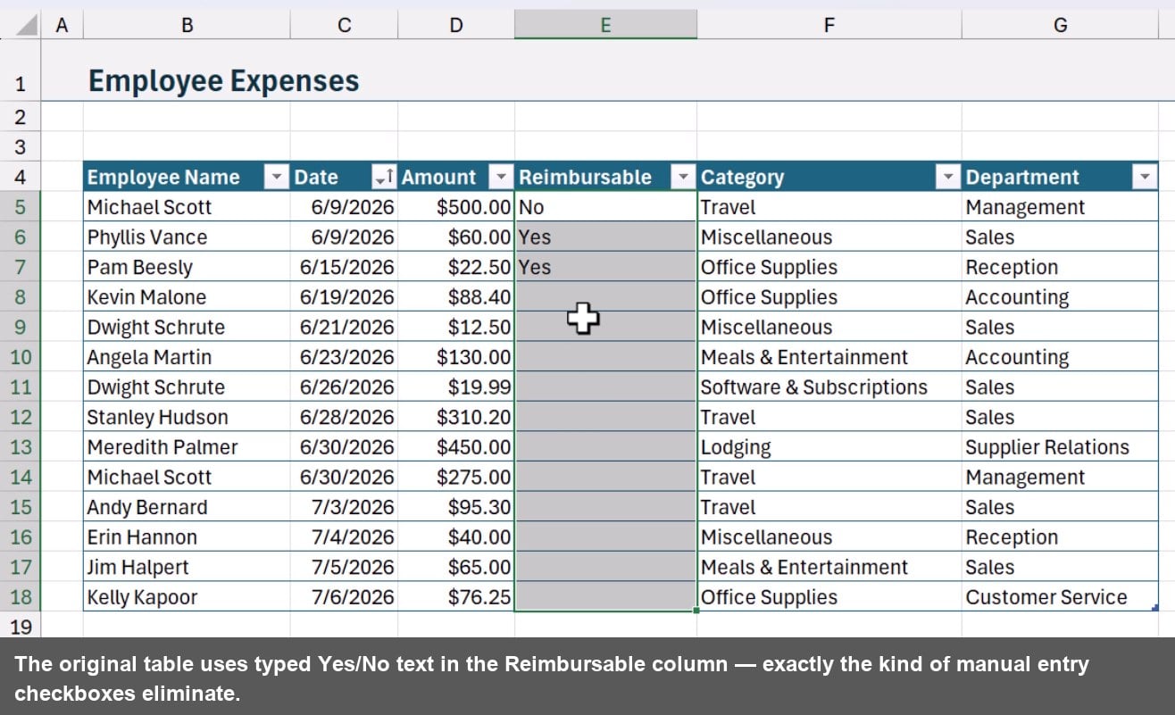
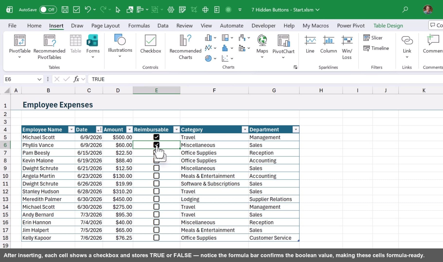
Checkboxes are available in Microsoft 365 (desktop and web). If you're on an older version, the next technique is a great alternative for controlled data entry.
Button 2: Data Validation Dropdown Lists
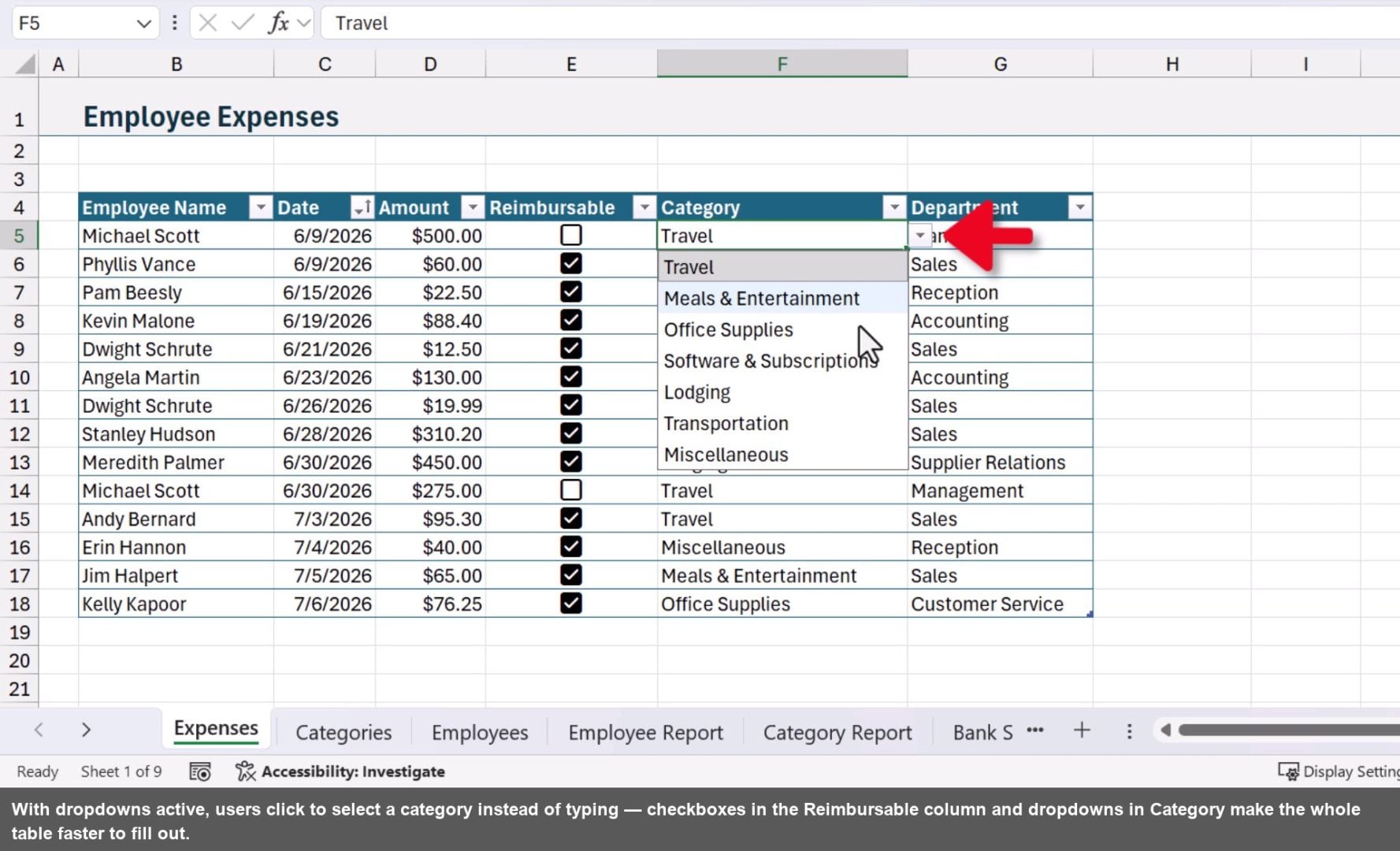
Freehand typing in a Category column is a recipe for mismatched data. One person types “Meals & Entertainment,” another types “Meals and Entertainment,” and your SUMIFS formula misses half the records. Dropdown lists lock the input to an approved set of values.
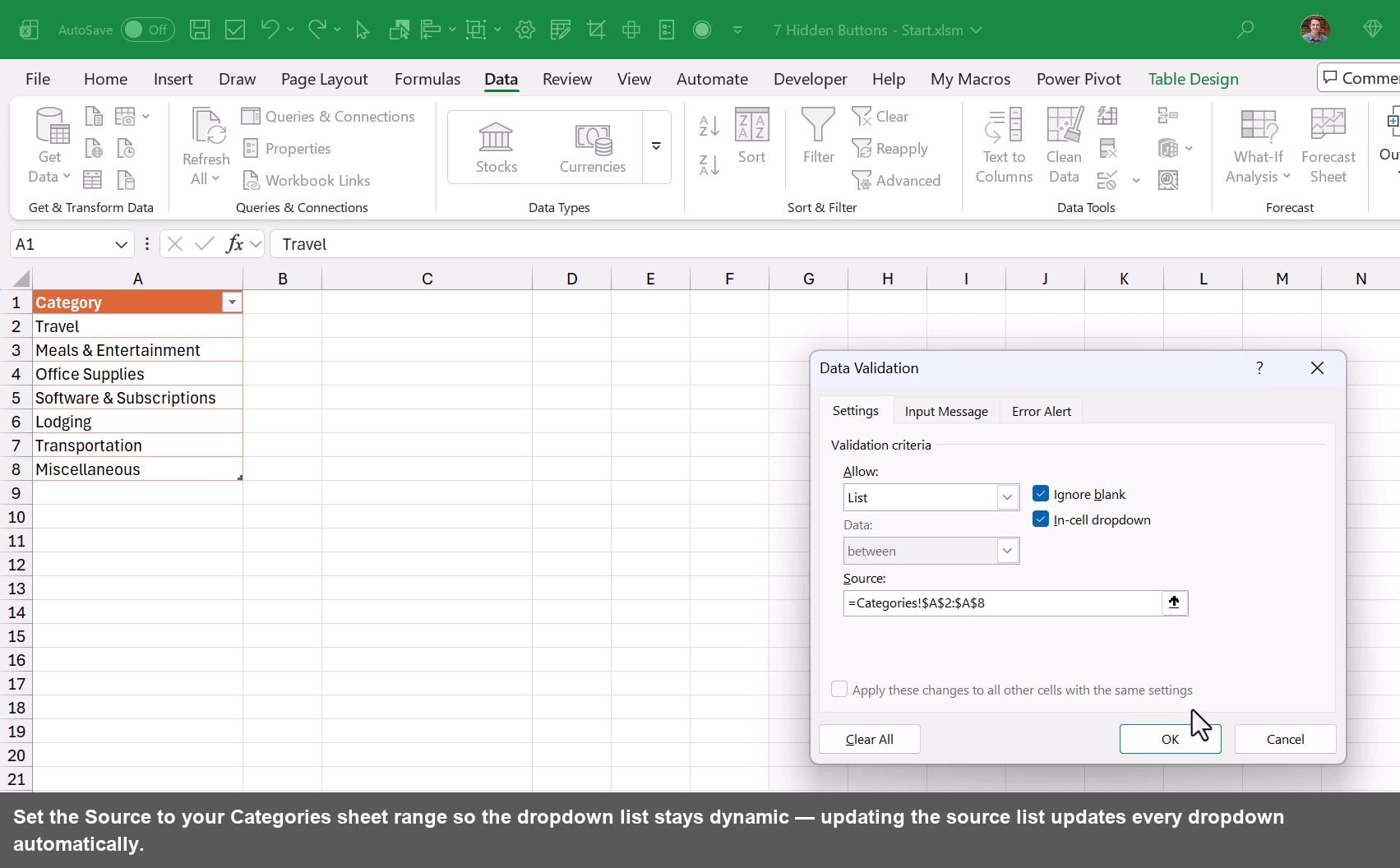
Select the cells in your Category column, go to the Data tab, and click Data Validation. Under Allow, choose List, then point the Source to your category list on a separate sheet. Any new rows added to the table automatically inherit the dropdown.
Button 3: Slicers for One-Click Filtering
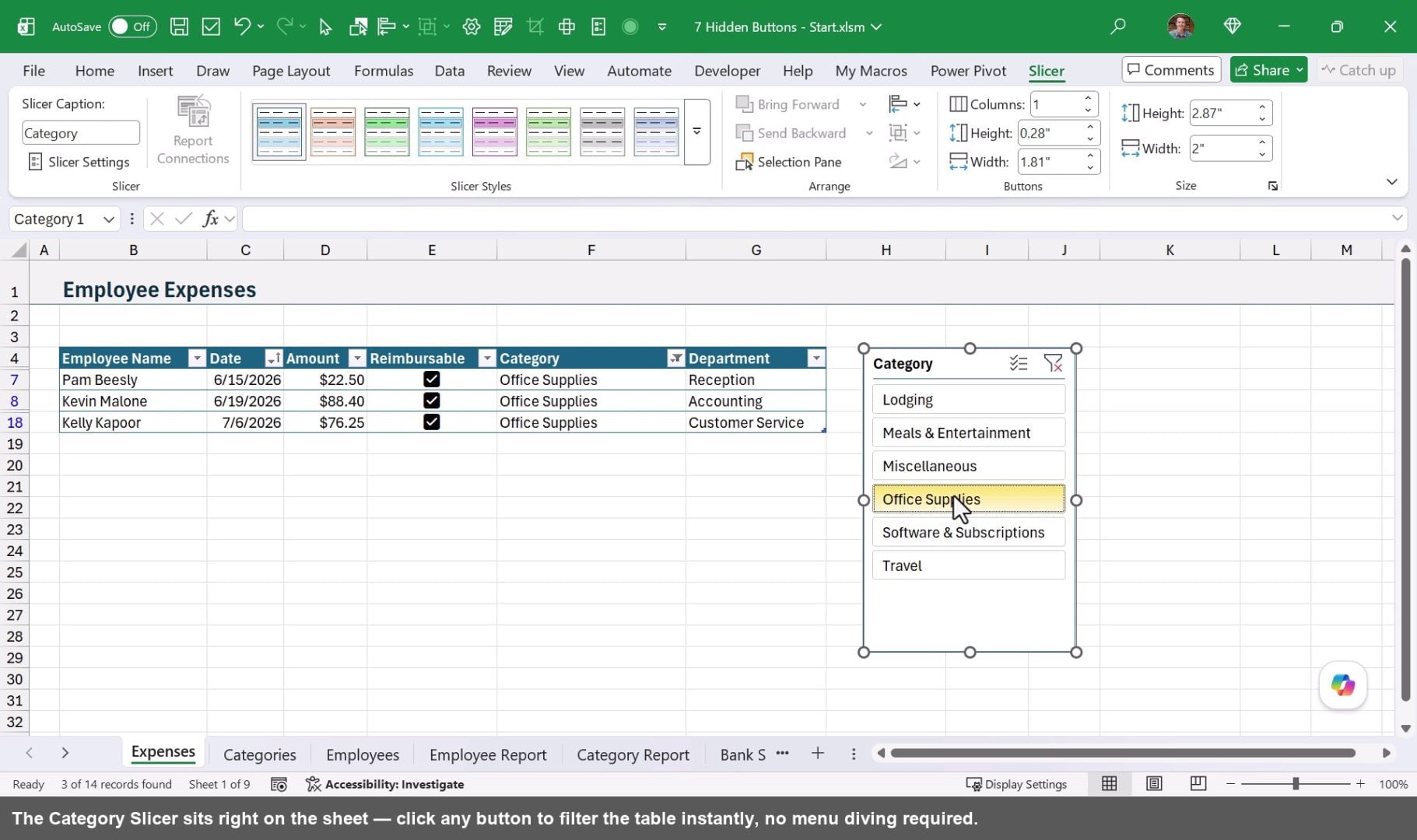
The standard table filter dropdown requires multiple clicks: open the menu, uncheck Select All, pick your item, click OK. A Slicer turns that into a single button click. Your data must be in an Excel Table first (Insert, Table), then go to Insert and click Slicer. Choose the field you want to filter by and click OK.
The Slicer appears as a panel of clickable buttons on the sheet. Click a category to filter, click the clear button to show everything again. Slicers also connect to Pivot Tables and Pivot Charts, making them a go-to tool for interactive dashboards.
Button 4: Navigation Shapes for Multi-Tab Workbooks
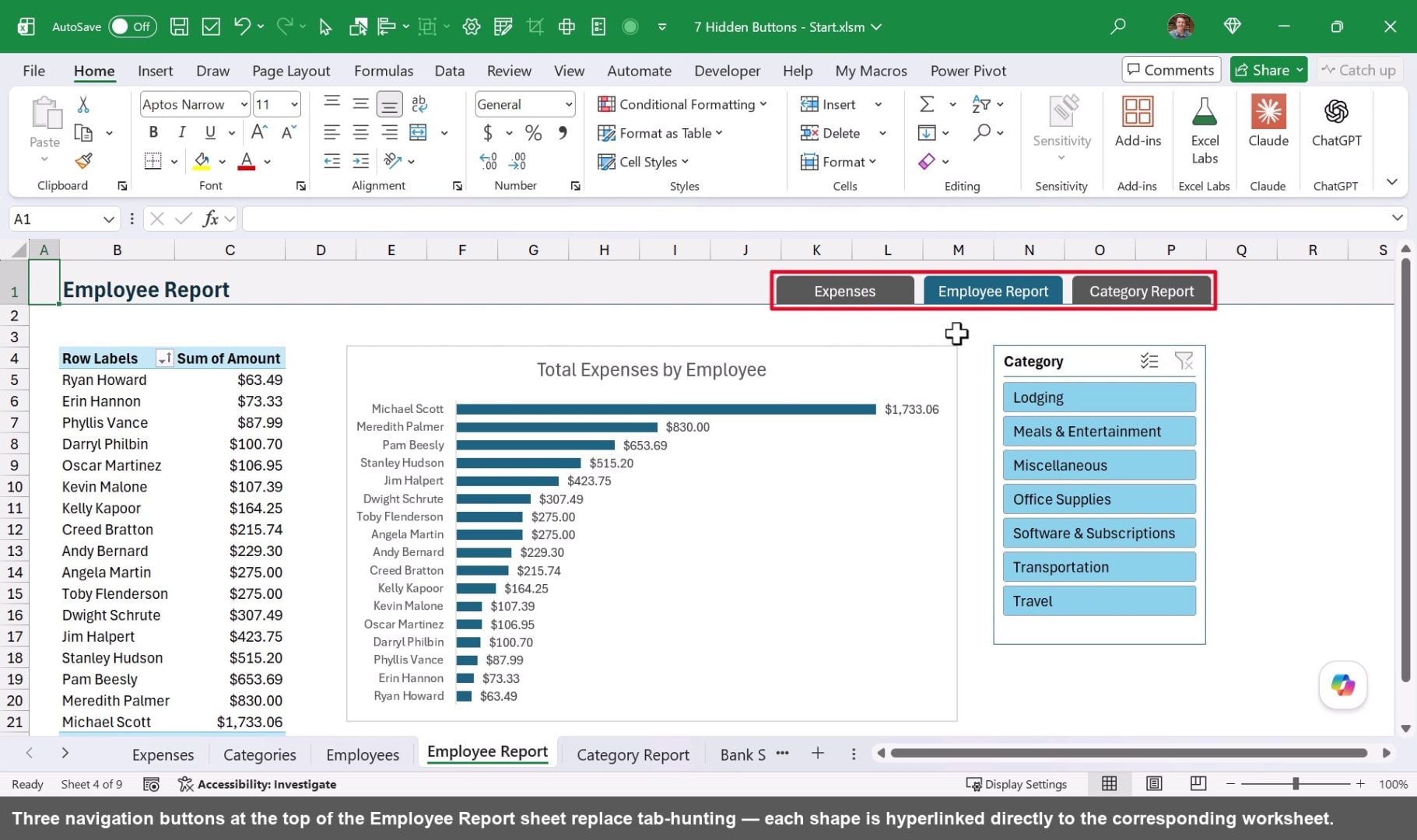
Scrolling through 9 sheet tabs to find the right report frustrates users. You can turn any shape into a navigation button. Go to Insert, Illustrations, Shapes, and draw a rounded rectangle at the top of your sheet. Type a label, then right-click the shape and choose Link.
In the link dialog, go to Place in this Document and select the target sheet. Click OK. Now clicking the shape jumps directly to that sheet. Add one button per report tab, and your workbook suddenly feels like a proper app.
Button 5: Macro Buttons and VBA UserForms
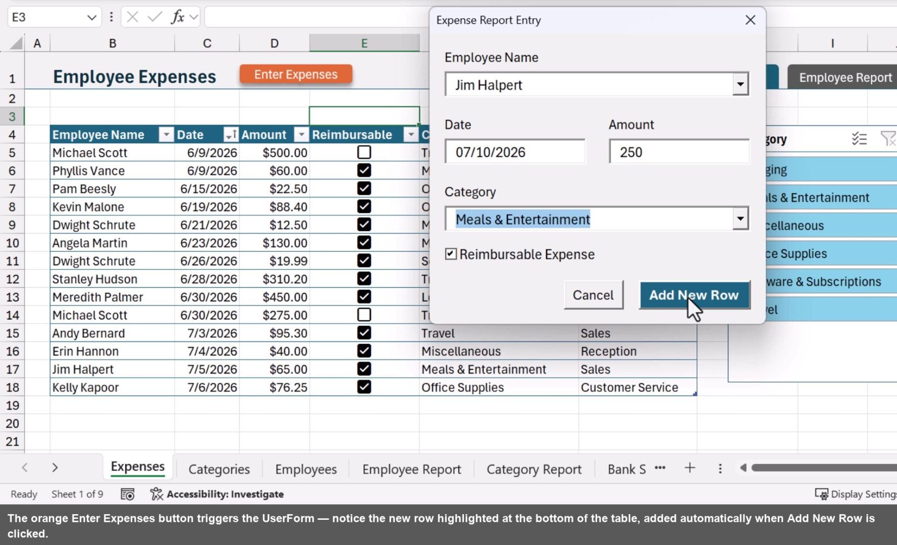
Shapes can also run macros. Right-click any shape, choose Assign Macro, select your macro from the list, and click OK. Now the shape is a clickable trigger for any automated process in your workbook.
In this example, the button opens a custom VBA UserForm for structured expense entry. The form includes dropdown lists, a date field, an amount field, and a checkbox for reimbursable status. Clicking Add New Row writes the entry directly into the table. These forms are fully customizable inside the Visual Basic Editor (Developer tab, Visual Basic button).
AI Coding for Excel Course
I explain more about creating macros and userforms in my AI Coding for Excel Course.

This course is designed to help you build real automation inside Excel using AI tools like Copilot, Claude, and ChatGPT. You'll unlock AI's superpower, writing code, to save HOURS with repetitive Excel and Office tasks.
The course covers three powerful coding languages: VBA, Office Scripts, and Python in Excel.
Button 6: Column and Row Grouping
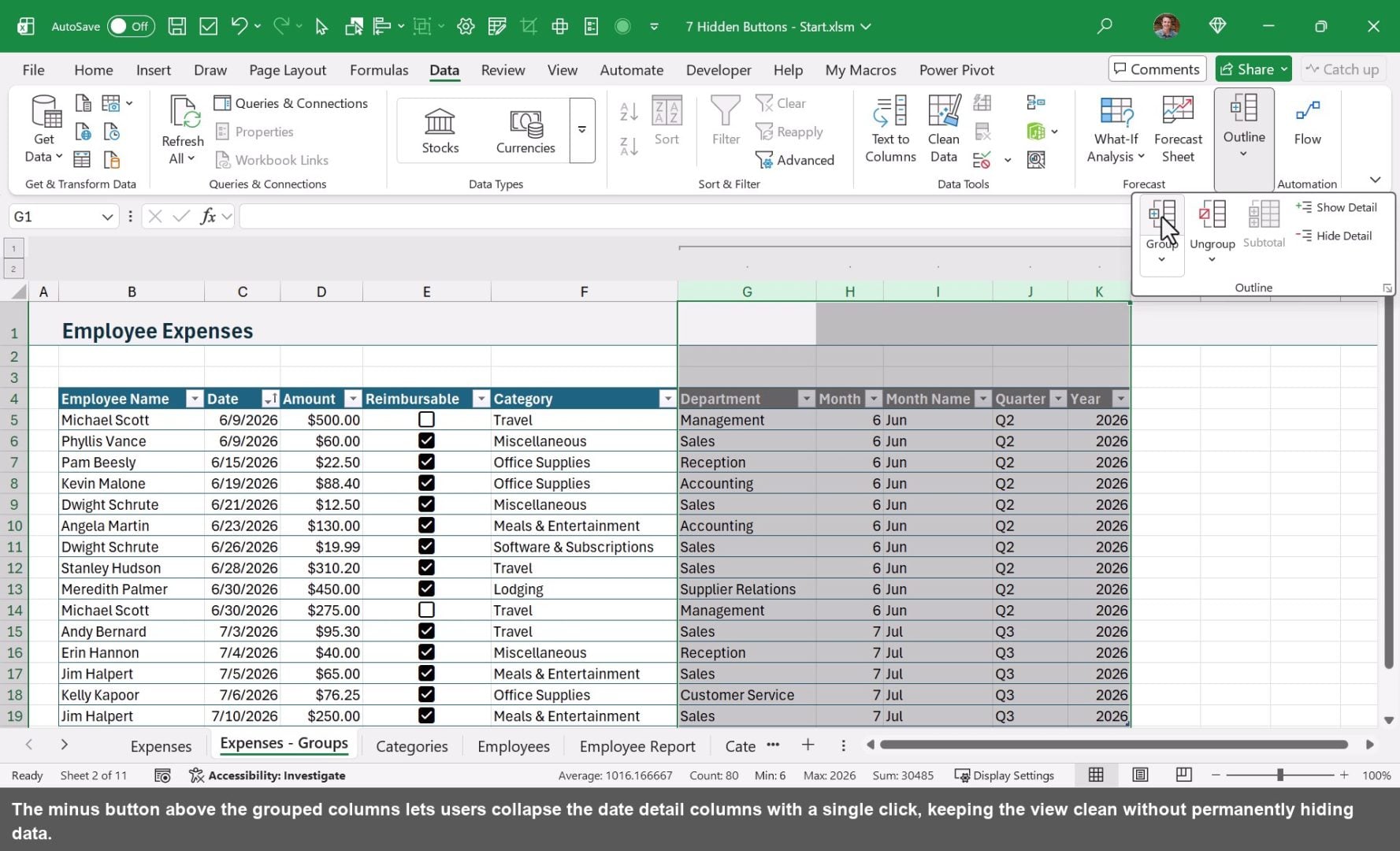
Hiding and unhiding columns through the right-click menu gets old fast. Grouping is a better approach. Select the columns you want to collapse, go to Data, and click Group. Excel adds a small minus button above the grouped columns. Click it to collapse the group, click the plus to expand it.
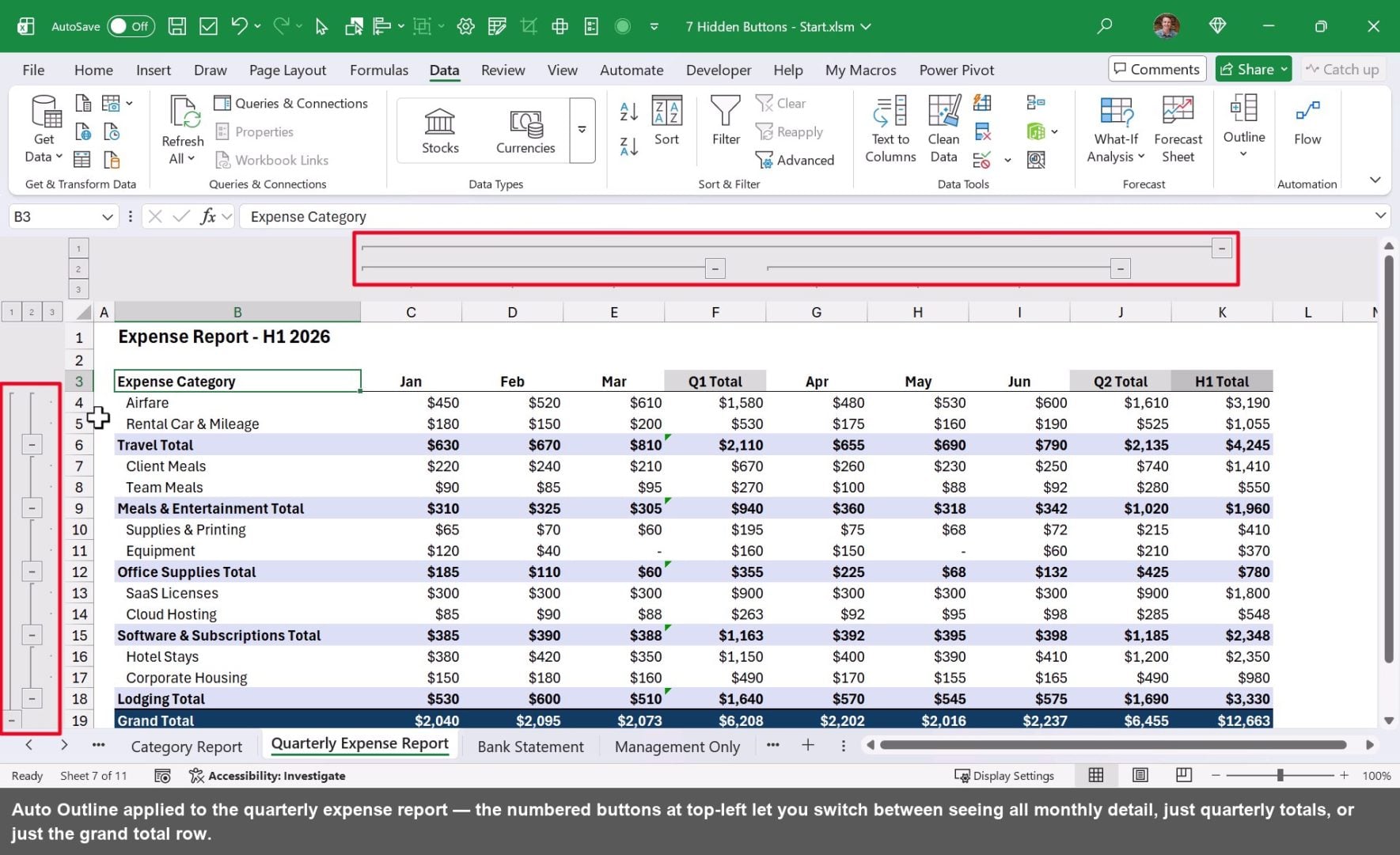
For structured financial reports with monthly detail and subtotals, use Auto Outline instead. Go to Data, Group dropdown, and choose Auto Outline. Excel analyzes the layout and creates groupings for both rows and columns automatically. The numbered buttons in the top-left corner let you expand or collapse all levels at once.
Button 7: Spin Buttons for Scenario Analysis
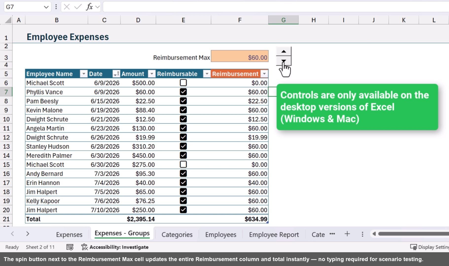
When someone needs to test different values repeatedly, like a reimbursement cap, making them retype a number every time slows things down. A Spin Button fixes this. You'll need the Developer tab first. If it's not visible, right-click anywhere on the ribbon, choose Customize the Ribbon, scroll down on the right side, check Developer, and click OK.
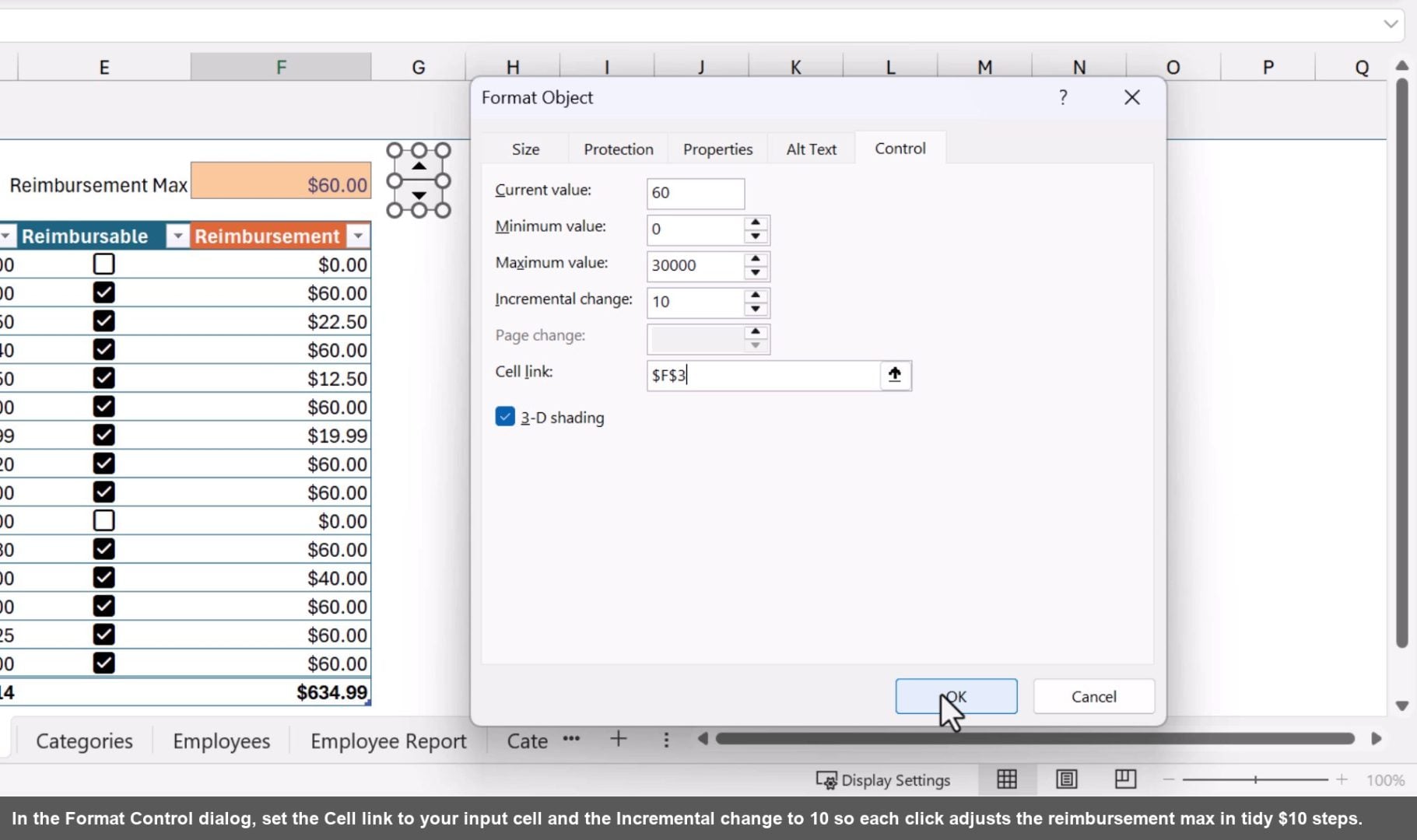
On the Developer tab, click Insert and choose the Spin Button control. Draw it next to your input cell. Right-click the button and select Format Control. Set your current value, min, max, and incremental change (10 in this example), then link it to your target cell. Now the up and down arrows increment the value without any typing.
Summary
Each of these seven buttons can make your spreadsheets more fun to use and easier navigate. Plus, they help prevent data entry errors and save time with repetitive tasks.
You don't necessarily need to add all seven to every single workbook. Start with the one that matches your biggest pain point today, and you'll immediately feel the difference.




Very nice videos as well as files templates too