Bottom Line: Learn how to use the COLUMNS function in VLOOKUP to prevent errors when inserting/deleting columns from your source range.
Skill Level: Intermediate
Video Tutorial
Download the Excel File
If you'd like to practice using the COLUMNS function in VLOOKUP using the same data I use in the video, download my file below.
Prevent VLOOKUP Errors When Columns Change
One limitation when using VLOOKUP is that it can easily return the wrong data when the information in the table array gets rearranged. Adding or deleting a column can mess up your data because VLOOKUP uses the column number when it formulates its answer.
For example, in this image below, you can see on the left that we've set up the VLOOKUP formula to return the email address for each of the names listed. The email address is found in the third column of the table array on the right.
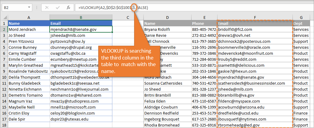
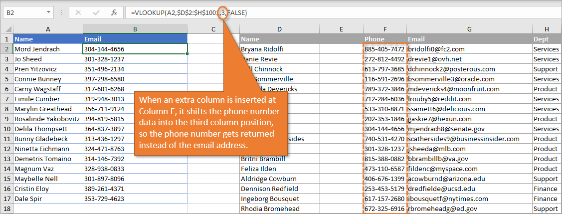
If we add or delete columns and shift those email addresses over, VLOOKUP will continue to return whatever data is found in the that third column.
The COLUMNS Function
There are several ways to fix this problem and the one I'm going to focus on in this tutorial is by using the COLUMNS function. This function returns the number of columns in an array or reference. To use the COLUMNS function just
- Type the equals sign (=) and begin typing the word “Columns.”
- Tab into the COLUMNS function (plural, not singular).
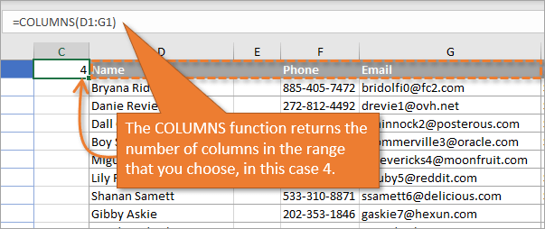
- Select your array. In the example below, I've selected from cell D1 to G1. Because there are four columns in that array (D, E, F, and G), the function returns the value of 4. As I add or delete columns in that array, that value will increase or decrease respectively.
So the COLUMNS function allows our reference to be dynamic. As columns in our range are added or deleted, that number remains the same. The number will identify the data we want because we end our array with the column we are interested in. There may be more columns of data, but we want to end our array with the column we are looking to use.
In our example, no matter how many columns we add or subtract in front of the email column, that column's number will always be the same as the total number of columns in our array (because it's the last column).
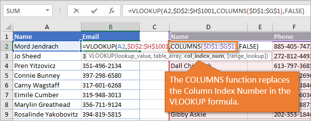
Replacing the Column Index Number
This formula that we've created can be used in place of the Column Index Number in our VLOOKUP formula.
One important step when selecting your array is to hit F4, which makes it an absolute reference. (Dollar symbols will be inserted in front of the row and column characters, indicating they are now absolute.)
Another good idea is to select the column headers (if there are any) when you are defining your range for the dynamic Column Index Number. That's because additions and deletions might be made to the data in the columns, but the headers are less likely to change.
By the way, the keyboard shortcut to add a column is Ctrl + + and the shortcut to delete a column is Ctrl + -. Checkout my post on 5 Keyboard Shortcuts for Rows and Columns to learn more.
Using the COLUMNS Function with Excel Tables
The COLUMNS function also works using ranges that are formatted as Excel Tables. The formula just looks more like this.
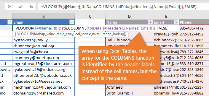
One advantage of using Excel Tables is that you can move columns around (within the existing parameters of the table data) and the VLOOKUP formula will still work correctly.
Pros & Cons
So, to summarize a bit, let me just outline some pros and cons of using the COLUMNS function in your VLOOKUP formula.
Pros
- This option is really easy to implement.
- Updating any existing VLOOKUP formulas is easy as well.
Cons
- The formula can break if columns are moved with regular ranges.
- Although moving columns still works with Excel Tables, you still can’t look to the left, or return a column to the left of the lookup column.
An alternative to avoid these cons is to use INDEX and MATCH and the new XLOOKUP, which you can learn more about in the tutorials outline below.
Related Tutorials
For a refresher on VLOOKUP and how it can be used, read my post called VLOOKUP Example Explained at Starbucks.
To see how the VLOOKUP and MATCH functions work together, read VLOOKUP & MATCH – A Dynamic Duo.
Alternatively, you can add the INDEX function into your repertoire to create more advanced formulas using INDEX and MATCH. Start by reading The INDEX Function – A Road Map For Your Spreadsheet.
If you are on Office 365, then you will be able to use the new XLOOKUP as well.
Conclusion
Setting up a dynamic reference for your Column Index Number helps to reduce formula errors when using VLOOKUP. If you have questions or comments, I look forward to reading them below.


Great solution john to use columns function making the column index argument in lookup more dynamic should colums be added or deleted.
Xlookup function sounds cool but in my case years away before implemented in my employers version of excel for windows. Will be a great addition when it arrives. Thanks for your helpful videos and explanations, they are so easy to understand which is the sign of an excellent tutor.
Thank you for the nice feedback, Richard! I really appreciate your support. 🙂
Hi Jon,
Thought this would be a useful time-saving tip along with a few variations.
By locking the column in both the lookup value and one corner of the “columns” formula, you can copy the formula across to populate your other column information.
=VLOOKUP($A2,$F$2:$I$1001,COLUMNS($F1:G1),0)
Alternatively, you could combine VLOOKUP with MATCH and hardcode the column header, which would be useful if you had a large spreadsheet and knew the column name, but not its position e.g.:
=VLOOKUP(A2,$G$2:$J$1001,MATCH(“Email”,$G$1:$J$1,0),0)
Furthermore, you could also do INDEX-MATCH-MATCH:
1)
=INDEX($H$2:$K$1001,MATCH(A2,$H$2:$H$1001,0),MATCH(C$1,$H$1:$K$1,0))
OR
2)
=INDEX($H$2:$K$1001,MATCH(A2,$H$2:$H$1001,0),MATCH(“Email”,$H$1:$K$1,0))
NB: the one proviso, if using a cell reference (1) as opposed to hardcoded value (2) ensure you use absolute or partial references, so the formula is always pointing to the same header and avoid #N/A errors.
Thanks,
Colin
Thanks Colin! Awesome tips! We actually have a separate video & post planned for this topic of copying Vlookup formulas across. You’re one step ahead of me. 😉
Hi Jon
I normally use Excel as an export function in my Access databases so my Excel abilities are very limited. Having said that, I find your videos and tips extremely useful and, most importantly, clear and relatively easy to understand. I very much appreciate your efforts.
I also want to congratulate you and your wife for the recent addition to your family… I couldn’t even tell that you are sleep deprived…
Hi Silvio,
Thank you for the nice feedback and your support. I really appreciate it. Coffee helps with the sleep deprivation and short bursts of energy needed to record videos. LOL!
Thank you very much for your explanations they are really useful. 🙂