Bottom Line: Learn how to create a formula that returns unique combinations of values from non-adjacent columns.
Skill Level: Intermediate
Watch the Tutorial
Download the Excel File
If you want to follow along, you can use this workbook. It's the same file I use in the video.
Pulling Unique Lists from Columns That Aren't Adjacent
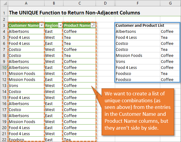
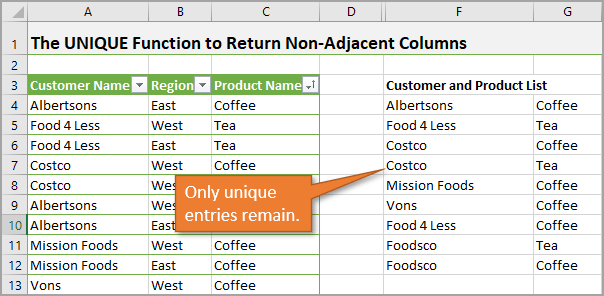
We received a great question from Irene, who is an Elevate Excel member. She's curious to know if the UNIQUE function can be used to pull entries from columns that are not side by side or next to each other.
The answer to Irene's question is: on it's own, the UNIQUE function can only find unique combinations from adjacent columns. However, we can write a formula to work around that. This formula will essentially create an array of the non-adjacent columns that you want to reference in the UNIQUE function.
It's a similar process to what I explained in this tutorial on the FILTER Formula to Return Non-Adjacent Columns in Any Order.
Here's how to write the formula we need:
Use INDEX to Create an Array for Non-Adjacent Columns
Below is an example where we want to use the UNIQUE function, which is a dynamic array function, to return a list of unique combinations of Customer Names and Product Names. As you can see, those two columns are not next to each other.
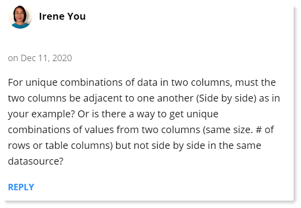
Since the UNIQUE function does not handle that on its own, we have to use use another formula to help. So we're going to use INDEX.
For the INDEX function, the first argument is the array. We will select the entire table for the array.
The next argument is row number (row_num). To define the row numbers we want, we'll first create a list of row numbers using the SEQUENCE function.
The first argument (and the only one we need) in SEQUENCE is rows. To define rows, we will actually use the ROWS function. The only argument for the ROWS function is array, and for that, we will again reference the entire table. This will return every row from the table to our new array.
To define the column number argument (column_num), we can reference column numbers as an array in curly brackets. In our case we want to pull from columns 1 and 3. Those column numbers are specific to the table we're working with, not the sheet overall.
So, all together, our formula to return an array of non-adjacent columns looks like this:
=INDEX(tblUnique,SEQUENCE(ROWS([tblUnique]),{1,3})
Wrap the Formula with UNIQUE
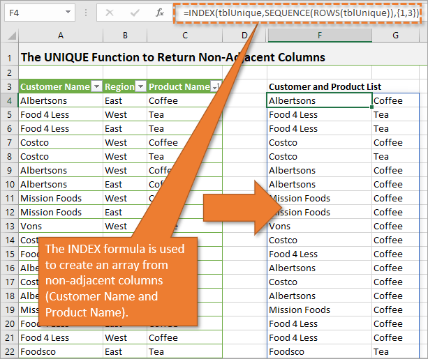
Now that we've created a spill range that shows the columns we want, we simply have to wrap our existing formula with the UNIQUE function.
The UNIQUE function has other arguments, but the only one we need to use is array. Our array is defined by the formula we already created. So the final formula looks like this:
=UNIQUE(INDEX(tblUnique,SEQUENCE(ROWS([tblUnique]),{1,3}))
With our duplicates filtered out, our spill range only shows unique entries from the two columns we wanted to pull from.
Conclusion
You can then sort the list of unique values by wrapping the formula in the SORT or SORBY function. Or you could further filter down the results with the FILTER function.
The possibilities are endless in terms of what you can do with dynamic arrays to create flexible, interactive reports. Checkout our video & post on Dynamic Array Formulas & Spill Ranges to learn more.
Please leave a comment below with any questions or suggestions. Until next time!


This good insight never thought of this. Thanks
Thanks Paul!
Can we also sort customer name and Product alphabatically?
This is really helpful! Could you take it 1 step further and look for counts of each of these unique combinations as well?
Thanks!
Hi Dan,
Great question! Yes, it is possible and there are several ways to go about it. With formulas you could use a COUNTIFS function.
=COUNTIFS(tblUnique[Customer Name],F4,tblUnique[Product Name],G4)
You could also use a pivot table to create the summary report.
I hope that helps. Thanks again and have a nice day!
Thank you Jon for this Video. I have a question. If I want to get the dates sequence , which is only Saturday& Sunday for 3 months. How can I do this?
Hi Rahul,
Great question! This is also possible with dynamic array formulas. Here is a formula that uses SEQUENCE and FILTER. It assumes the start date is in cell M5 and end date in M6.
=FILTER(SEQUENCE(M6-M5,,M5),WEEKDAY(SEQUENCE(M6-M5,,M5),2)>5)
We’ll add this formula to our list for future videos. The SEQUENCE function has a lot of uses with dates.
Thanks!
Hi, thank you so much for this! How could i take it step further and add a filter . For example, return these UNIQUE columns only when column C= “apples”
Hi Jon,
why i dont have SEQUENCE and UNIQUE function?
Hi Jon
Thanks for sharing you can also use the CHOOSE function to join ranges together like this.
=UNIQUE(CHOOSE({1,2},A2:A6,D2:D6))
I can’t find Sequence function in Excel 2019. Is it replaced by some other function in this version of excel?
This is very helpful. If i want to sort in descending order, then what should be the formula. Thanks
You just reverse the values in the arrays. So where Jon used “{1,3}” to get columns A and C in that order, you’d use “{3,1}” to get them in the reverse order (C, then A).
Works the same for the rows. Just make the array in reverse order to have the bottom row at the top and so on.
If using SEQUENCE instead of writing the arrays out, do it in the last two of its four arguments. For instance, the following would create the array {1,3,5,7,9}:
SEQUENCE(5,1,1,2)
but this would get the reverse ( {9,7,5,3,1} ):
SEQUENCE(5,1,9,-2)
Older ways of creating these arrays used things like “ROW(1:3)” and that took a different technique. One said, OK, that’s 3 rows, so if I take the array ( {1,2,3} ) it creates and subtract it from one value higher (“4”), then I’d have the array {3,2,1} and INDEX() would turn the table upside down. Then a VLOOKUP() or similar thing would get the latest record for a match, not the earliest one. (Can’t do “ROW(3:1)” because Excel changes it, no matter what, to “ROW(1:3)”… so… thanks, Excel.
Doesn’t work in Google Sheets. Use QUERY instead. For ex. UNIQUE(QUERY(A1:C10;”select A, C”))
You don’t need to use QUERY to do this in google sheets, just two ranges within another array {brackets}
=UNIQUE({A1:A10,C1:C10})
Hopefully, Excel will develop something like this one of these days.
Hi, how can I make the 1 and 4 in this formula below (which are in “{ }” refer to cell inputs? I can only get it to work with “{1,4}” actually typed in the INDEX formula. Ideally I’d like the 1 and 4 to be MATCH() results.
=INDEX(A1:D10,SEQUENCE(ROWS(A1:D10)),{1,4})
I’ve tried “{“&1&”,”&4&”}” – with 1 and 4 being cell results, but can’t get it to return the 2 arrays that the typed {1,4} gives.
I’m using this to create a single array from 2 non-adjacent arrays to be used in LINEST as the independent variables (allowing multiple regression) against a given dependent variable array.
Thanks
Excel does not permit building an array constant from string materials as you are trying.
If you can figure a way to generate such an array constant from a function it would work. Excel creates many internal-to-the-calculation array constants when evaluating formulas and that would just be “one more.” But since it would really be an array constant, not a string-building construct, it would do the job.
I’m not saying whatever function you use will be naturally intuitive or even seem “natural” in any way, but it will work. For example, say you are working with the formula you present, and you use XMATCH (or MATCH, both will produce an array constant if set up like this):
=INDEX(A1:D10,SEQUENCE(ROWS(A1:D10)), XMATCH({1,4},{1,0,0,4},0))
You’d have to type it and get that typing right, but you have to do that to build a string anyway so the effort’s a wash. For most, you might even be able to “automate” the internal array constant that is typed here (the “{1,0,0,4}”) the same way-ish that ROWS “automates” the SEQUENCE function used in the formula.
For that, and a more complex array constant, one might just enter a formula like:
=IF(a1=”x”,COLUMN(),0)
in row 2 of a sheet, for however many columns that there are in your INDEX’ed table/range. In A3, place the formula:
=ARRAYTOTEXT(A2:(whatever column)2).
In row 1 place an “x” in any column you need.
Notice the formula in A3 is the exact value you need for your XMATCH from above. Copy it, “Paste|Special|Values” in an easy cell, edit that cell (F2) and copy it all to the Clipboard. Paste that string of the array constant into your XMATCH and you built it rather than typed it.
And get rid of the helper stuff, of course. (Or maybe keep it in a “Useful Things” spreadsheet.)
Is there a similar way to do it with non-adjacent rows?
It doesn’t seem to work, as the sequence function has a mandatory row argument, but I need only the column argument. I want the unique headings of two difference tables (which are themselves results of data-based filtering).
Use “1” for the row argument.
For example, if A1:C9 has data in the odd rows and odd columns and you wish to have a tight little table with no blank rows (the even ones in this case) or columns (so, losing column B in this case), the following would do the trick:
=INDEX(A1:C9,SEQUENCE(5,1,1,2),SEQUENCE(1,2,1,2))
In it, the row argument SEQUENCE() will return 5 rows starting with row 1 and then adding 2 each iteration to get 3, 5, 7, and 9. That’s the “1,2” at the end. The 5 rows is obvious: the “5” it starts with. Seems perfectly natural for the column argument to be a “1” doesn’t it? After all, you are just wanting to specify rows in this argument so a simple “1” in the columns argument of SEQUENCE() makes it plain vanilla.
Same idea when working with the columns SEQUENCE() function: except here, it’s the rows argument that needs to have no impact on things so you use a “1” for it, then a real value for the columns (“2” since you want the 2 columns that have data), and finish it off with the start value (“1” for column 1) and the jump value (“2” so it gets column 3, not column 2).
So if you use SEQUENCE() on a row related argument, in INDEX() or anything else, you use a “1” in the columns value for it so the only variable has to do with rows. And the other way around if creating an array relating to columns (use the “1” in the rows argument so only the columns argument of SEQUENCE() is doing anything special).
(That’s just inside functions needing row and column related arrays. Lots of other times, you’d be happy to use “non-1” values in both!)
how to add sumifs formula in below formula
=UNIQUE(INDEX(tblUnique,SEQUENCE(ROWS([tblUnique]),{1,3}))
how can we add Sumifs from different sheet
=UNIQUE(INDEX(tblUnique,SEQUENCE(ROWS([tblUnique]),{1,3}))
Hi, I have tried both methods (index and choose) but I only have 1 column of data. Do you know why?
FYI the formula you have in your post is incorrect in that it doesn’t close the sequence function. It’s correct in your screenshot.
You have:
=INDEX(tblUnique,SEQUENCE(ROWS([tblUnique]),{1,3})
Should be:
=INDEX(tblUnique,SEQUENCE(ROWS([tblUnique])),{1,3})
Everything else is great, thanks for posting.
This can be done using the Filter command rather than the Sequence.
=UNIQUE(FILTER(tblUnique,{1,0,1}))
where the {1,0,1} tells it to include the 1st & 3rd columns.
Each of the 2 shown formulas is missing one closing parentheses. Will try to figure out how to correct.D
What about:
=UNIQUE(HSTACK(…))
?
thank you