FILTER Formula to Return Non-Adjacent Columns in Any Order

Bottom Line: Learn how to return a limited number of columns that are not in the original order with the FILTER function in Excel.  Also discover how to make the formula dynamic to prevent errors when inserting and deleting columns.

Skill Level: Advanced

Watch the Tutorial

Download the Excel File

Practice this technique on your own using the file that I use in the video. Download it here:

A Note About Dynamic Array Formulas

The Dynamic Array Formulas used in this post are only available for the latest version of Excel for Microsoft Office 365. Here is a post that explains more about Dynamic Array Formulas & Spill Ranges.

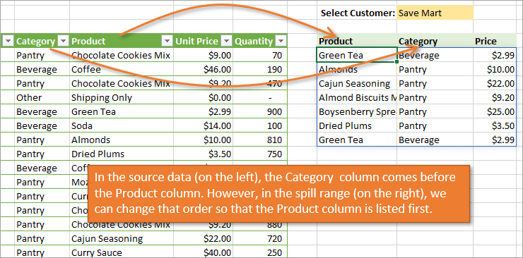
Returning Specific Columns in Any Order

If you've started using the awesome new FILTER function, then you might have run into the scenario where you only want to return a specific number of columns in an order that is different from the source range/table.

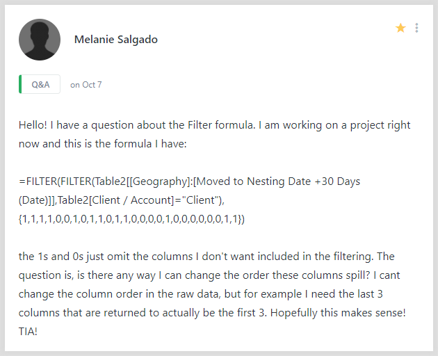
This was a great question from Melanie, a member of our Elevate Excel Training Program. She found a solution that allowed her to return individual columns, but they had to be in the same order as the source range.

One easy solution is to move the columns in the source range/table so that they are adjacent to each other. However, that is not always ideal or possible if you have multiple FILTER formulas for the same source range.

The good news is that we can use the INDEX function to create an array of non-contiguous or non-adjacent columns in an order that is different from the source data, which I explain in this post & video.

I also explain a technique for using a drop-down lists for the headers of the spill range so that you or your users can quickly change the columns that are returned.

Writing the Formula

Here is an example of the entire formula:

=FILTER(INDEX(tblData,SEQUENCE(ROWS(tblData)),{4,3,5}),tblData[Customer Name]=I3)

This can easily look complex or overwhelming when you first see it. However, we are just using an INDEX formula for the array argument of FILTER to create an array of non-adjacent columns. So let's look at that first.

The INDEX Formula Explained

The INDEX allows us to return an array or range of values to FILTER. INDEX has three arguments.

=INDEX(array,row_num,col_num)

Typically when you use INDEX you only specify one row number and one column number. However, we can also specify a list of numbers to return multiple rows and columns in a spill range.

There are two ways we can specify the list of row and column numbers in the INDEX arguments.

1. Using a formula like SEQUENCE or XMATCH to create the list.
2. In an array of hardcoded values in curly brackets: {1,2,3}

We are going to use both techniques in this formula.

1. Creating a list of Row Numbers with SEQUENCE

For the row_num argument of INDEX we need a list of all of the rows in the source range or table.

The SEQUENCE function will create this list for us. We only need to specify the rows argument in SEQUENCE and it will create a list from 1 to the number of rows specified.

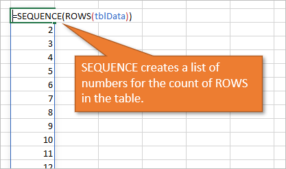
We can use the ROWS function to return the count of the number of rows in the source range or table.

So, here is the formula for the row_num argument in INDEX:

=SEQUENCE(ROWS(tblData))

There are currently 80 rows in the tblData table, but this formula will automatically update as rows are added or deleted from the table.

2. Specifying the Columns to Return

For the col_num argument of INDEX we can specify the column numbers we want to return. For this array we can use the list of column numbers in curly brackets. We can also specify the order of the columns to return.

The following array will return columns 4, 3, and 5 from the table in that order.

{4,3,5}

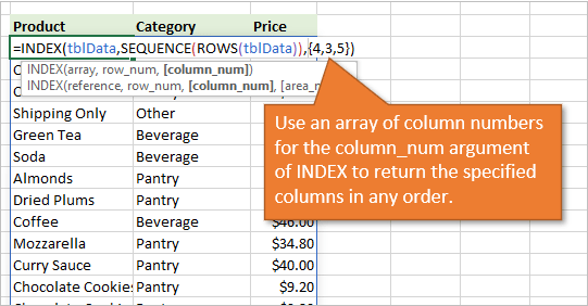
So, the following formula will create an array of all the rows and only three columns from the tblData table.

=INDEX(tblData, SEQUENCE(ROWS(tblData)), {4,3,5})

The FILTER Formula Explained

The INDEX formula we created above is used for the array argument in FILTER.

=FILTER(array, include, [if_empty])

The include argument is used to specify the filter criteria, or rows to return from the array.

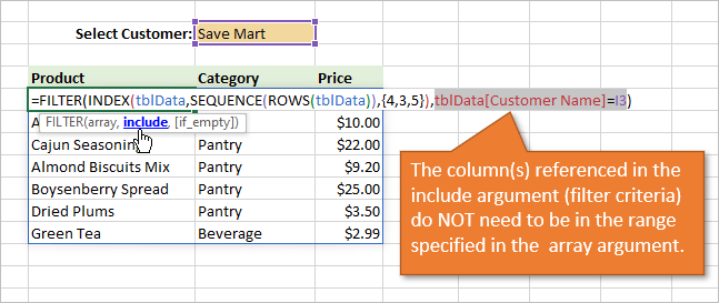
The great part about FILTER is that the column(s) you specify in the include argument do NOT need to be in the array. In the following example, the include argument is filtering the rows for a specific Customer Name. However, the Customer Name column is not included in the array that is returned by INDEX.

=FILTER(INDEX(tblData,SEQUENCE(ROWS(tblData)),{4,3,5}),tblData[Customer Name]=I3)

You can still use all the same techniques for specifying multiple criteria in the include argument. There are no limitations there. We do have dedicated training section on the FILTER function, including multiple criteria, in our Elevate Excel Training Program.

Avoiding Formula Errors with XMATCH

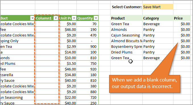
One issue that will eventually arise with this solution is when columns are added or deleted from the source data table. The formula will return values we don't want because we hardcoded those column numbers in the curly brackets. Those hardcoded values {4,3,5} will NOT change when the source table/range is modified.

To avoid this issue, we can replace the hardcoded list with an XMATCH formula.

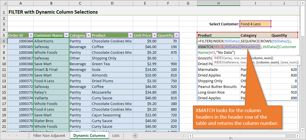
The XMATCH function will do a lookup for the column headers that we specify above the spill range of FILTER, and return the column numbers of each column in an array (list). XMATCH returns a list because we are specifying a range of multiple cells in its lookup_value argument.

Here is the XMATCH formula:

XMATCH(H5:J5,tblData[#Headers])

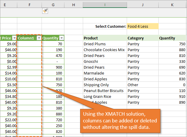
Now when you add or delete columns from the table, XMATCH will automatically update to return the new column numbers based on the lookups that it performs.

A side benefit of this technique is that it also makes it easy to add columns to the results of the FITLER formula. You can just add a new column header in a blank cell to the right of the headers, then adjust the XMATCH formula to include that cell in the lookup_value range.

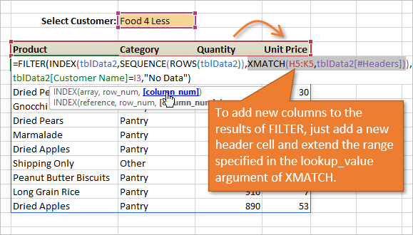
The spill range for FILTER will extend to the right with that one simple change.

Make it Interactive with Drop-down Lists

With the XMATCH function in place, one way to really make this list dynamic and interactive is to add drop-down lists to our headers. Then we can change the headers to any column name and the column will automatically update to return the respective column.

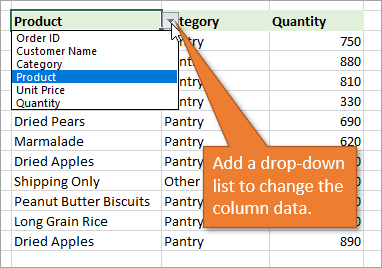
This means that you or the users of your file can quickly change the columns that are displayed in the resulting spill range of FITLER. There is essentially no maintenance or refresh required to make those changes. In other words, our arrays are very dynamic. 😉

Here's a tutorial on how to create those drop-down lists with the UNIQUE function: How to Create a Dynamic Drop-down List that Automatically Expands.

Conclusion

So that's how you change the column order of your return array. I admit that this solution is a bit complex. It may take some time to really study and understand each component, but it sure makes for a fantastic interactive end-result.

This is also a great example of how powerful and useful the new Dynamic Array Formulas truly are.

If you have questions or suggestions, I encourage you to leave a comment below.

Thanks again and have a great week! 🙂