Bottom line: Learn time-saving tips that will help you write, modify, and audit formulas in Excel.
Skill level: Beginner
Video Tutorial
Formula Tips
We probably spend the majority of our Excel lives writing and modifying formulas. They are the heart of Excel, and amazingly powerful!
Formulas can also be frustrating, overwhelming, and difficult to figure out. So, in this post I share five tips & shortcuts to help you read and write formulas faster.
#1 – Enter & Edit Modes with F2
When you have a cell selected, pressing the F2 key puts the cell in Edit mode. If the cell contains a formula, you will see the formula in the cell and be able to edit it. This is the same as double-clicking the cell with the mouse.
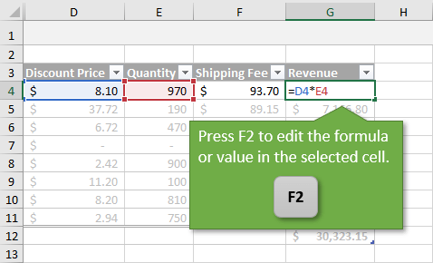
But there's more to it…
Sometimes you might want to select a cell/range with arrow keys to change a reference. When you press the arrow keys in Edit mode, the text cursor moves within the formula.
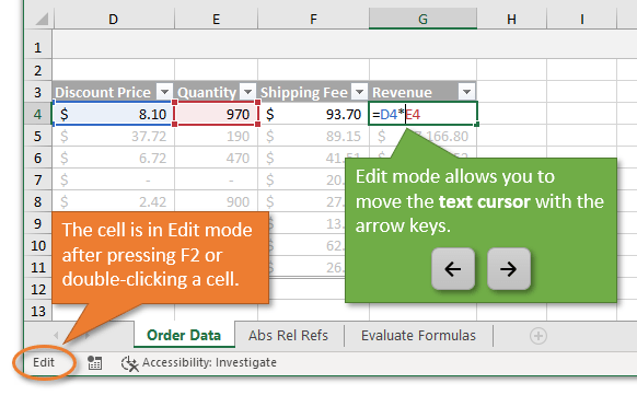
At this point you can press F2 again to put the formula in Enter or Point mode. Now the arrow keys will select cells instead of moving the text cursor.
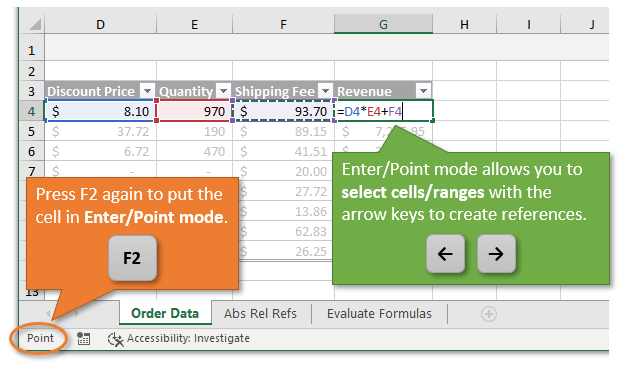
The mode is displayed in the bottom-left corner of the application window in the Status Bar.
You can press F2 again to toggle back to Edit mode, to move the text cursor. This toggle allows you to modify formulas by just using the keyboard.
The use of F2 will depend on the scenario. Sometimes it's faster to use the mouse. However, Enter & Edit modes make it very easy to select text or ranges with shortcut keys like Ctrl+Shift+End.
Checkout my articles on 5 Keyboard Shortcuts for Rows and Columns in Excel and 2 Keyboard Shortcuts to Select a Column with Blank Cells to learn more tips for selecting ranges.
#2 – Absolute & Relative Reference with F4
If you find yourself typing the $ symbol to create absolute/relative references, then the F4 key will quickly become your new best friend.

After creating a range reference in a formula (with either the mouse or keyboard), pressing the F4 key will add the $ symbols and make the reference absolute.
The F4 key is a toggle that will cycle through all absolute, mixed, and relative reference states.
- 1st press – Full Absolute Reference: $A$2
- 2nd press – Absolute Row Reference: A$2
- 3rd press – Absolute Column Reference: $A2
- 4th press – Full Relative Reference: A2
You can continue to press F4 to cycle through these states. The cycle will start at the existing state for the reference and change to the next when you press F4.
F4 also works on range references ($A$2:$A$10).
When you first create the reference by selecting it with the mouse or keyboard, press F4 to make apply the change to the full reference.
If you modify an existing range reference then you will need to select the entire reference before pressing F4. Otherwise it will only modify the part of the reference that the text cursor is in.
I share a quick way to select the entire range reference in the next tip
#3 – Select Argument Text with Screentip Hyperlinks
Sometimes it's difficult to find and modify arguments within complex formulas. We can use the function's screentip hyperlinks to help with this.
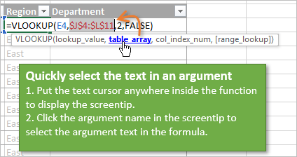
When you put the text cursor inside a function, a screentip appears below with the function's arguments. Click the hyperlink for any argument to select the argument's text in the formula.
If you are modifying the absolute/relative reference of the formula, then you can press F4 directly after clicking the link.
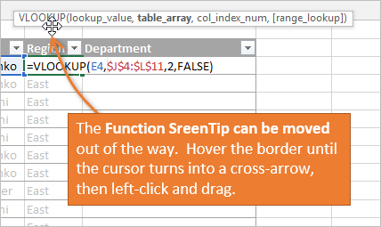
Bonus tip: If the function screentip is in your way, you can also move it by hovering the mouse over the border until the cursor turns into a cross arrow.
#4 – Evaluate Formula Components with F9
When dealing with long and complex formulas, you might want to see the results of a nested function/formula (a formula within the formula).
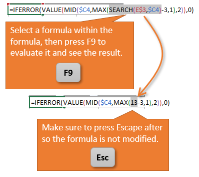
Select the text within the formula that you want to evaluate, then press the F9 key. Excel will calculate the selected text and return the result direct to the formula.
This can help you step through and understand how a formula calculates, but there are a few important things to know.
- You must select the entire expression or function. If you only select part of a function's text then Excel will show an error message.
- Press Escape after evaluating parts of the formula. This is important! Escape will exit out of Edit mode and not commit the changes.
If you press Enter then the results of the evaluation will be committed to the formula, and you will lose the parts of the formula you evaluated.
The F9 shortcut works well when you are trying to figure out what a specific component of the formula is calculating. The next tip explains how to step through the entire formula.
#5 – The Evaluate Formula Window
The Evaluate Formula Window is a great tool if you've inherited a workbook that contains complex formulas. It allows you to step through each component of the formula and see how it calculates.
Here's how to use it.
- Select the cell that contains the formula you want to evaluate.
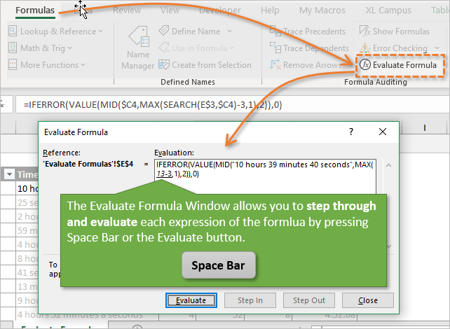
- Go to the Formulas tab in the Ribbon and press the Evaluate Formula button. (keyboard shortcut: Alt, T, U, F)
- The Evaluate Formula window will appear with the formula loaded in the Evaluation box.
- The underlined expression within the formula will be evaluated next.
- Press the Evaluate button, or the Space Bar, to evaluate the expression and see the result in the formula.
- You can continue to press Evaluate or Space Bar to evaluate each step.
- You will eventually see the result of the entire formula. You can then press Restart or Space Bar again to start over.
- You can close the window at any time during the evaluation process. The window does NOT change the formula at all.
If you find yourself stepping through the formula several times, then you might want to switch back to editing the formula and use the F9 shortcut. I often use both of these techniques when learning or debugging a complex formula.
Function Lock on Laptop Keyboards
At the end of the video I mentioned a tip if the function keys (F1-F12) are not working for you. This is typically due to your keyboard having multi-purpose function keys, which is common on laptops and smaller/newer keyboards.
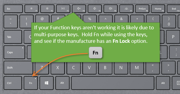
If that's the case, you will have to press the Fn key in combination with the function key. This can definitely slow you down!
Fortunately, many keyboards have an Fn Lock feature that allows you make the function keys the primary command. You can usually do a quick Google search with the model name of your keyboard/laptop and the phrase “fn lock”, to see if it is available. All manufactures handle this differently.
As a last resort, you can also modify the BIOS to lock the function keys. This is not a permanent change, but harder to toggle on/off quickly.
Checkout my article on the Best Keyboards for Excel Keyboard Shortcuts to learn what to look for in a keyboard. I also share the keyboard I use in that article.
Conclusion
I hope these tips help save you time when working with formulas. This is by no means an exhaustive list.
Please leave comment below with any additional tips or shortcuts you use when working with formulas. Thank you! 🙂


Hi Jon,
It’s Sumon from Bangladesh. I have a functional problem. I want to multiple a Minimum value from a table with another cell. but I filed to do this by MIN function.
=IFERROR(P6<=1,"",((MIN(IF($C$5:$C$39=$N6,$E$5:$E$39)*P6))))
It's my formula. please help me to solve my problem.
Thank you
Hi Sumon,
IFERROR() only needs 2 arguments, IF() needs 3
there is also the MINIFS() formula which might help you:
= MINIFS ( $E$5:$E$39, $C$5:$C$39, $N6 ) * P6
might be what you are looking for (you may also want to check your $ signs!)
and I prefer not to use IFERROR() as it often masks bad formulae
jim
Hi. I’m trying to comment on the other post but it says can’t find the page or following an expired link. Did anything change?
I mean the convert text to dates page – I wanted to share a user defined formula that solved the problem
This article is of great help!
I have a question for something that does not seem to have been covered on this blog. I have an income and expenses spreadsheet with tabs for each month. I created multiple links that link to the respective places on the same worksheet. My problem is when I create a new month and copy the sheet to that new month the links do not work as they are still linked to the original sheet. I can edit the links individually to work in the new sheet but that is a long a tedious task. Is there a way I can edit all the links at once or some other solution when making a copy to get the links to work on the new sheet.
Hi Ian,
I suspect you have named ranges in your formulae?
I shudder to recommend this but converting them to A1 references is the simplest way – there are better solutions, but that should be a quick fix
The best solution is don’t use a different-tab-per-month format for recording data in the 1st place: put all your data in a flat format table and have a report tab that looks at that for a selected time period
jim
Hi Jon, great article! Is there a way to increase the size of the window/font of the function’screentip? The font is pretty small (which is quite annoying). Thanks for coming back on this.
Windows Magnifier?
Great tips! I especially found the shortcut for editing formulas directly in the cell really helpful. Can’t wait to try these out in my spreadsheets!
Great tips! I especially found the use of keyboard shortcuts to quickly navigate and edit formulas incredibly helpful. It’s amazing how such small changes can improve workflow. Thanks for sharing!
Great tips! I especially found the formula troubleshooting techniques helpful. I often get stuck on complex formulas, and the step-through evaluation method will definitely save me time. Thanks for sharing!
Great tips! I especially found the advice on using named ranges really helpful for keeping my formulas organized. Can’t wait to implement these in my next project! Thanks for sharing!
Thanks for sharing these tips! I especially found the trick for using named ranges really helpful. It’s such a game changer for keeping my formulas organized and easier to read. Looking forward to more Excel insights!
Great tips! I especially found the section on using named ranges really helpful. It’s such a time-saver when working on large spreadsheets. Thanks for sharing!
Great tips! I’ve been using Excel for years and didn’t realize how much quicker I could edit formulas with these techniques. The keyboard shortcuts are especially helpful. Thanks for sharing!